Lecture 13 – Applications of Machine Learning in CFD and GFD

What Is Learning

Falsifiability is fundamental to learning. If a theory is falsifiable then it is learnable – i.e. admits a strategy that predicts optimally. An analogous result is shown for universal induction.

A theory that explains everything, [predicts] nothing.

Reference: Falsifiable ⟹ Learnable

What Is Machine Learning

The goal of machine learning is to make computers “learn” from “data”. From an end user’s perspective, it is about understanding your data, make predictions and decisions. Intellectually, it is a collection of models, methods and algorithms that have evolved over more than a half-century now.

Machine Learning vs Statistics

Historically both disciplines evolved from different perspectives, but with similar end goals. For example, Machine Learning focused on “prediction” and “decisions”. It relied on “patterns” or “model” learnt in the process to achieve it. Computation has played key role in its evolution. In contrast, Statistics, founded by statisticians such as Pearson and Fisher, focused on “model learning”. To understand and explain “why” behind a phenomenon. Probability has played key role in development of the field.
As a concrete example, recall the ideal gas law $PV = nRT$ for Physics. Historically, machine learning only cared about ability to predict $P$ by knowing $V$ and $T$, did not matter how; on the other hand, Statistics did care about the precise form of the relationship between $P, V$ and $T$, in particular it being linear. Having said that, in current day and age, both disciplines are getting closer and closer, day-by-day.

Machine Learning vs Artificial Intelligence

Artificial Intelligence’s stated goal is to mimic human behavior in an intelligent manner, and to do what humans can do but really well, which includes artificial “creativity” and driving cars, playing games, responding to consumer questions, etc. Traditionally, the main tools to achieve these goals are “rules” and “decision trees”. In that sense, Artificial intelligence seeks to create muscle and mind of humans, and mind requires learning from data, i.e. Machine Learning. However, Machine Learning helps learn from data beyond mimicking humans. Having said that, again the boundaries between AI and ML are getting blurry, day-by-day.

Neural Networks and Deep Learning

In the early days of artificial intelligence, problems that were very difficult for human intelligence but relatively simple for computers, such as those that could be described through a series of formal mathematical rules were quickly solved. The true challenge of AI lies in tasks that are easy for humans to perform but hard to formalize, such as recognizing spoken language or faces in images. For these tasks, humans often rely on intuition to solve them effortlessly.
Ironically, abstract and formalized tasks are among the most mentally demanding for humans, yet they are the easiest for computers.
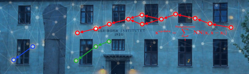
Neural networks (NNs) were inspired by the Nobel Prize winning work of Hubel and Wiesel on the how visual processing of cats starts with simple structure( ex. oriented edges) and brain builds up the complexity of the visual information until it recognizes the complex visual world. Their experiments showed that neuronal networks were organized in hierarchical layers of cells for processing visual stimuli. NobelCat

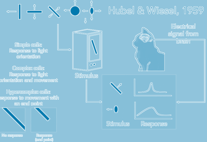
(An experiment where a cat sees different images or stimuli. Credit: Ho Jin Lee.)

Based on the original judgment, more criteria are added to distinguish between different details, in order to arrive at the most reasonable conclusion, this is deep learning.
The recent success of NNs has been enabled by two critical components:

the continued growth of computational power
exceptionally large labeled datasets

NNs specifically optimize over a compositional function $$ \overbrace{ \underbrace{\arg\min_{A_j}}_{\text{optimization over network weights}} \left[ f_M(A_M, \dots, f_2(A_2, f_1(A_1, x)) \dots ) + \underbrace{\lambda g(A_j)}_{\text{regularization term}} \right] }^{\text{overall neural network training objective}} $$ For deep learning models, instead of optimizing individual weight matrices $A_1, A_2, \dots, A_M$ at each layer, deep learning frameworks bundle all parameters into a single vector or set $\theta$: $$ \arg\min_\theta f_\theta(x) $$ where $\theta$ are the neural network weights and $f(\cdot)$ characterizes the network (number of layers, structure, regularizers).
It can be seen that the learning process in deep learning becomes a problem of finding the parameters $\theta$ that minimize a loss function over data: $$ \arg\min_\theta \mathbb{E}_{x \sim \mathcal{D}} \left[ \mathcal{L}(f_\theta(x), y) \right] $$

Machine Learning in Computational Fluid Dynamics

The heavy computational load and long runtimes of numerical simulations:

time-series-based prediction (machine learning can be a solution)

Risk: prediction errors accumulate over time, eventually causing the model to break down. The number of time steps it can sustain varies from a few dozen to a few hundred, depending on the type of flow condition and the initial/boundary settings.

Predicting certain features at specific time points or under steady-state conditions directly from the input boundary/initial conditions

Risk: the biggest challenge lies in obtaining a high-quality training dataset

Fluid motion is extremely complex and difficult to predict accurately (machine learning is not an easy fix)

Unless your training set comes from high-quality experimental measurements. But such data is expensive to obtain and often subject to noise and random error.

Flow phenomena include both open and closed systems, with various shapes. The system boundaries include moving/stationary walls as well as velocity/pressure inlets and outlets. These flows include vertical motion under gravity and planar flows in zero gravity. Their flow characteristics encompass the formation of viscous boundary layers, vortex formation and shedding, and jet development. They include both single-phase and two-phase flows, as well as laminar and turbulent regimes.
[Ex] Four representative classic CFD problems: (1) Cavity Flow, (2) Tube Flow, (3) Dam Flow, and (4) Cylinder Flow
CFDBenchSketch

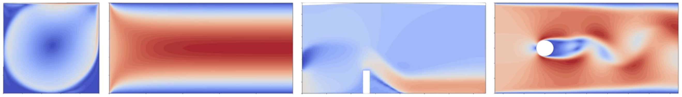Reference: CFDBench

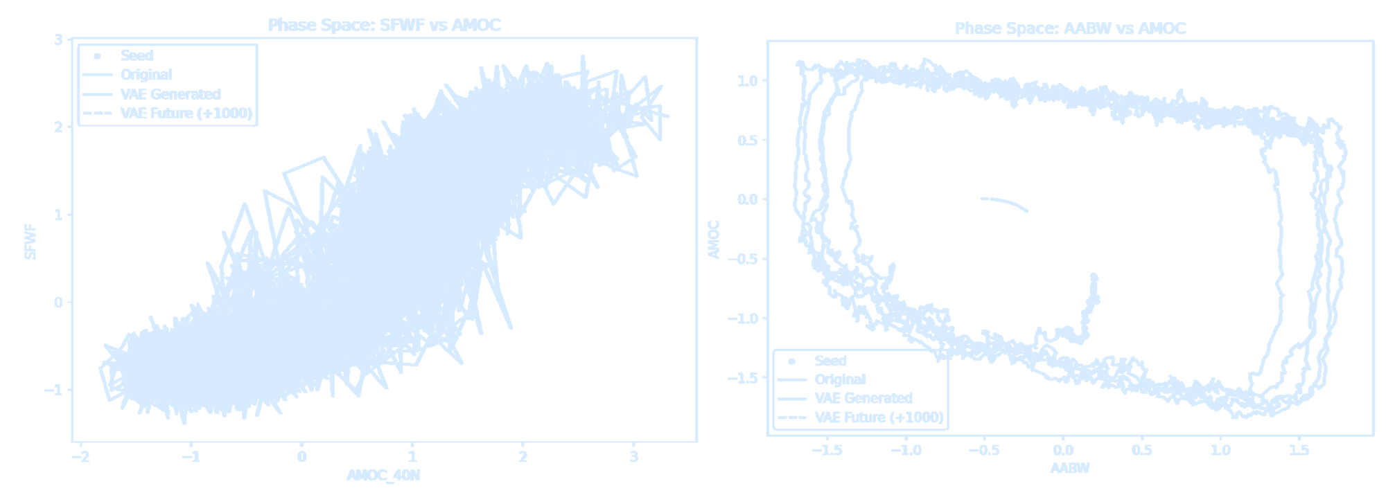
Machine Learning in Geophysical Fluid Dynamics

See Digital Worlds by TeamOcean!

Data-Driven Dynamical Systems

Consider dynamical systems of the form $$ \frac{d}{dt} \mathbf{x}(t) = \mathbf{f}(\mathbf{x}(t), t, \boldsymbol{\beta}) $$ where $x$ is the state of the system and $f$ is a vector field that possibly depends on the state $x$, time $t$, and a set of parameters $β$. For example, consider the Lorenz equation: $$ \begin{aligned} \dot{x} &= \sigma (y - x), \\ \dot{y} &= x(\rho - z) - y, \\ \dot{z} &= xy - \beta z \end{aligned} $$ In this case, the state vector is $$ \mathbf{x} = \begin{bmatrix} x & y & z \end{bmatrix}^T $$ and the parameter vector is $$ \boldsymbol{\beta} = \begin{bmatrix} \sigma & \rho & \beta \end{bmatrix}^T $$

import numpy as np
import matplotlib.pyplot as plt
from scipy.integrate import odeint

# Parameters for Lorenz system
rho = 28.0
sigma = 10.0
beta = 8.0 / 3.0
dt = 0.01

# Define the Lorenz system
def f(state, t):
    x, y, z = state
    return sigma * (y - x), x * (rho - z) - y, x * y - beta * z

# Initial state and time steps
state0 = [1.0, 1.0, 1.0]
time_steps = np.arange(0.0, 40.0, dt)

# Solve the system
x_train = odeint(f, state0, time_steps)

# Plot x vs z
plt.figure(figsize=(6, 4), facecolor='none', dpi=300)
plt.plot(x_train[:, 0], x_train[:, 2], color='#d6ebff')
plt.plot(x_train[0, 0], x_train[0, 2], "o", color="#d6ebff", markersize=8)
plt.gca().set_facecolor('none')
plt.gca().spines['top'].set_color('#d6ebff')
plt.gca().spines['right'].set_color('#d6ebff')
plt.gca().spines['bottom'].set_color('#d6ebff')
plt.gca().spines['left'].set_color('#d6ebff')
plt.tick_params(colors='#d6ebff')
plt.xlabel("x", color='#d6ebff')
plt.ylabel("z", color='#d6ebff')
plt.grid(False)
plt.show()

# Plot each dimension over time
def plot_dimension(dim, name):
    fig = plt.figure(figsize=(9, 2), facecolor='none')
    ax = fig.gca()
    ax.set_facecolor('none')
    ax.plot(time_steps, x_train[:, dim], color='#d6ebff')
    ax.spines['top'].set_color('#d6ebff')
    ax.spines['right'].set_color('#d6ebff')
    ax.spines['bottom'].set_color('#d6ebff')
    ax.spines['left'].set_color('#d6ebff')
    ax.tick_params(colors='#d6ebff')
    ax.set_xlabel("time", color='#d6ebff')
    ax.set_ylabel(name, color='#d6ebff')
    plt.grid(False)
    plt.show()

plot_dimension(0, 'x')
plot_dimension(1, 'y')
plot_dimension(2, 'z')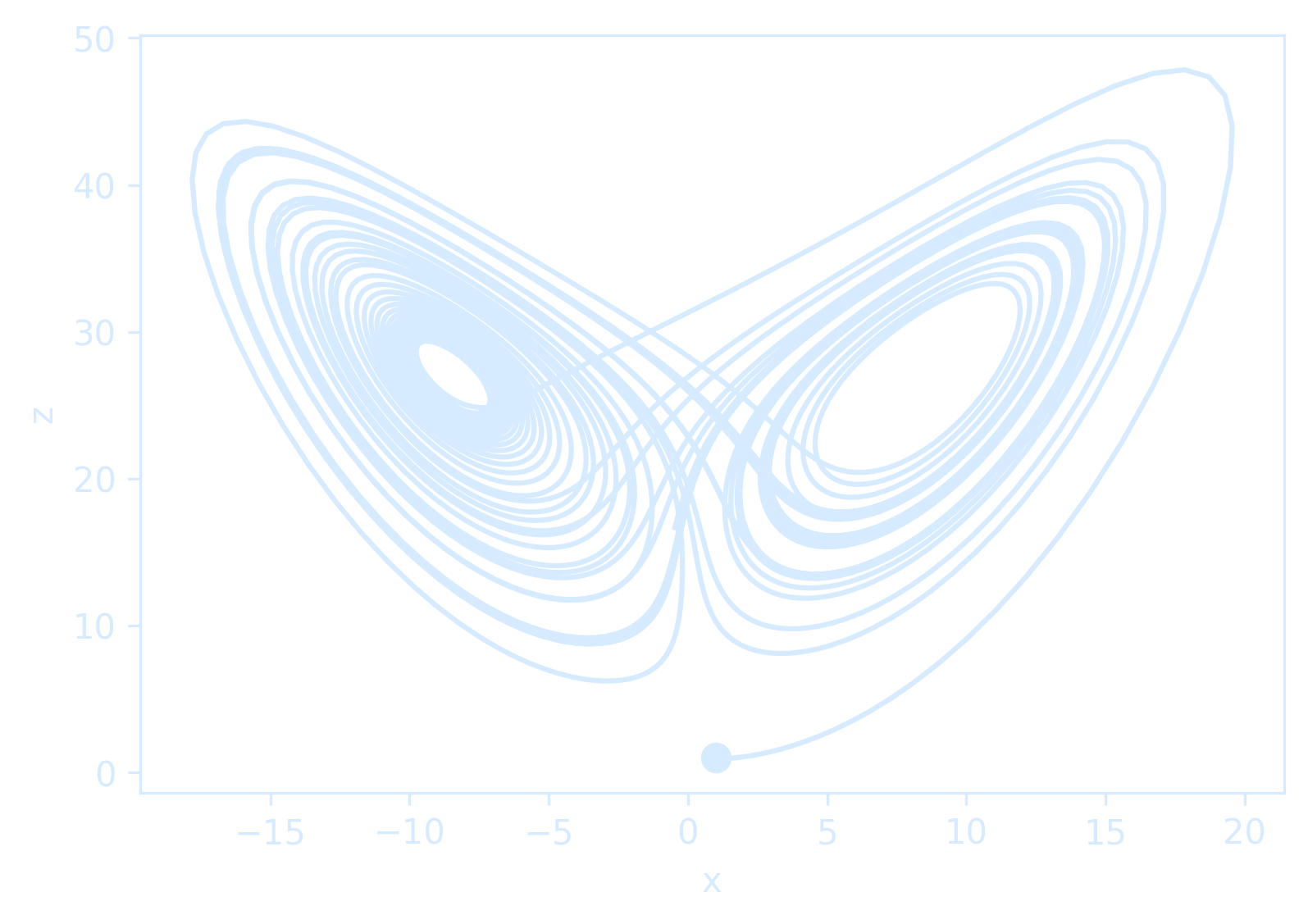

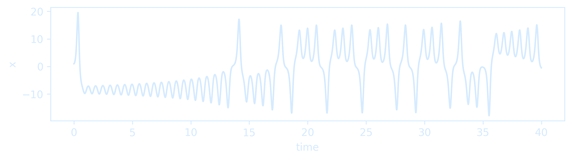
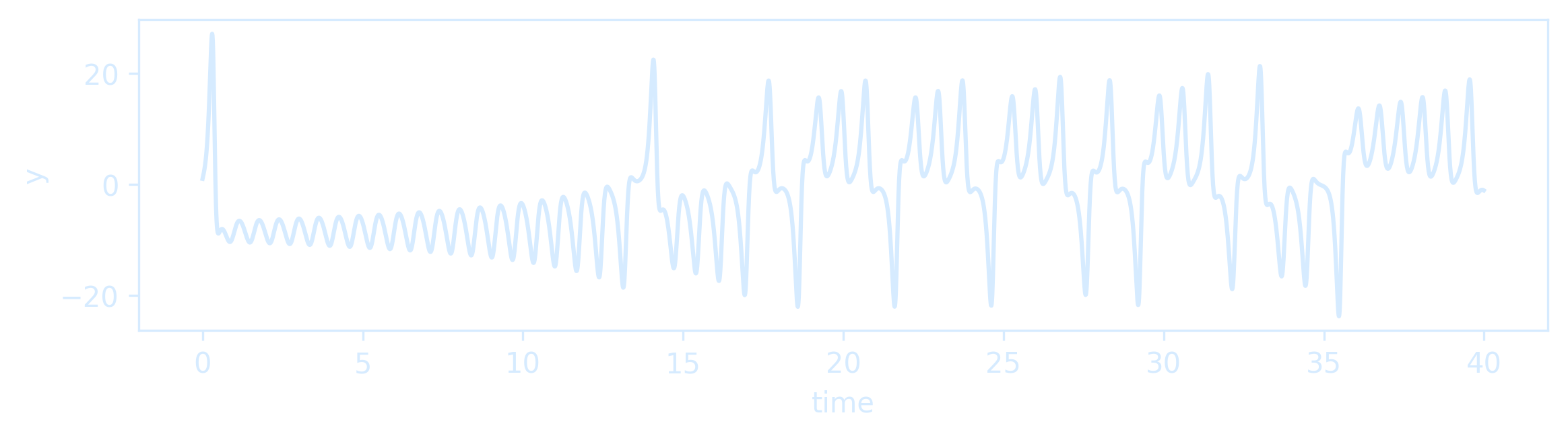
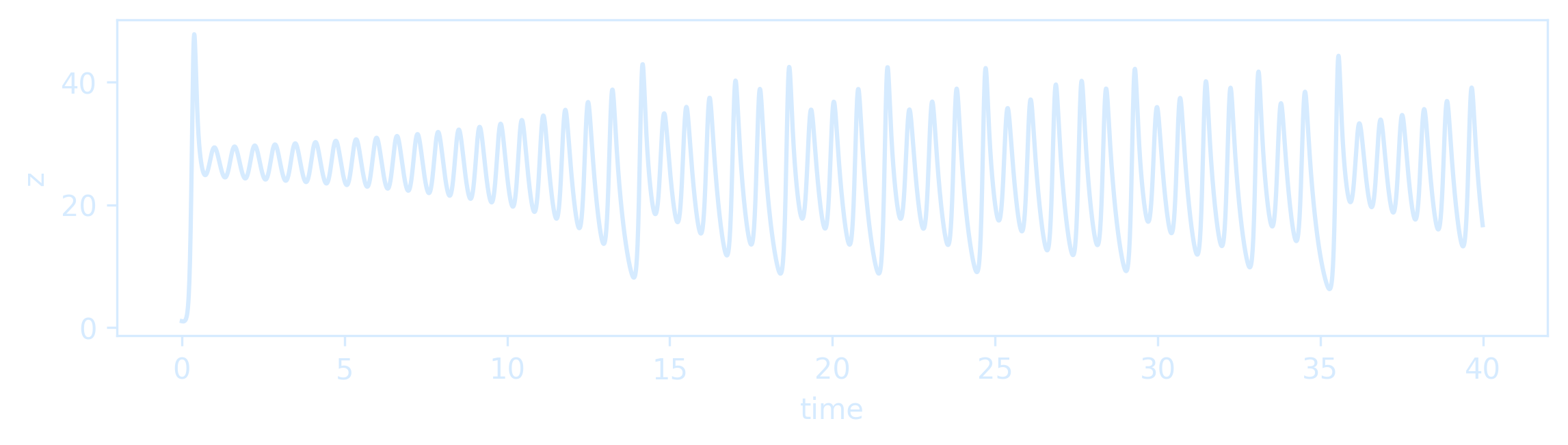The Lorenz system is among the simplest and most well-studied dynamical systems that exhibit chaos, which is characterized as a sensitive dependence on initial conditions. Two trajectories with nearby initial conditions will rapidly diverge in behavior, and, after long times, only statistical statements can be made. It is simple to simulate these dynamical systems, such as the Lorenz system.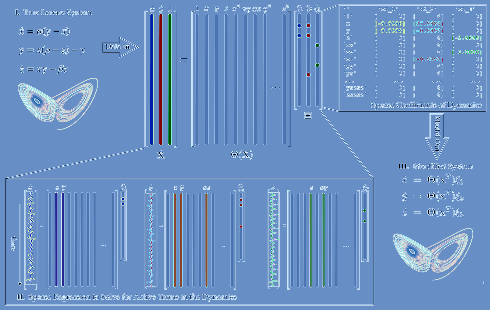

But more is different. SnowFlakesFractal

See Introduction to Dynamical Systems and Chaos to read more about bifurcation, chaos, and fractals.

Neural Networks for Dynamical Systems

NNs offer an amazingly flexible architecture for performing a diverse et of mathematical tasks. If sufficiently rich data can be acquired, NNs offer the ability to interrogate the data for a vairety of tasks centered on classification and predictions.
NNs can also be used for fitire state predictions of dynamical systems. We are now trying to build NNs trained on trajectories to advance the solution into the fitire for an arbitary initial condition. We are now trying to build NNs trained on trajectories to advance the solution into the future for an arbitrary initial condition. PhaseSpaceAMOC

Neural Ordinary Differential Equations

In a typical neural network the hidden state is represented as a series of discrete transformations: \[ h(t+1) = f(h(t), \theta(t), t) \] where $\theta$ is a parameterized hidden layer neural network: \[ h(t+1) = \sigma (\mathbf{W}_t h(t) + b_t), \] but $t$ can also be interpreted as continuous time. In this case, transitioning the input $x$ at $t=0$ to the output at $t=N$ involves a sequence of transformations.
However, one issue with this view is that it assumes the variable transitions are discrete, whereas many real-world systems, such as physical simulations, evolve continuously rather than through discrete updates. Thus a more reasonable choice is to model this problem as an Ordinary Differential Equation (ODE): \[ \frac{d h(t)}{d t} = f(h(t), \theta(t), t) \] From another perspective, instead of directly modeling $h(t)$, we might attempt to model its change rate $\frac{d h(t)}{d t}$.
Differential equations have been studied for centuries, and many numerical solvers exist to approximate their solutions. Instead of treating $h(t)$ as a function to be optimized, we can view it as a process to be solved. Given an ODE and an initial state $h(t_0)$, we can solve for the continuous-time function $h(t)$ over any time interval $t \in \mathbb{R}$.
Assume that the final output state is $h(t_1) = y$, the loss function can be defined in terms of the ODE solver: \[ \mathcal{L} (h(t_1)) = \mathcal{L} (\text{ODESolve}(h(t_0), f, t_0, t_1, \theta)) \] which can be rewritten as: \[ \mathcal{L} \left(h(t_0) + \int_{t_0}^{t_1} f(h(t), t) dt \right) \] So Neural ODEs are treating the entire timeseries as a continuously (non-discretely) varying dynamical system. The world in the end is a continuum. EularNeuralODE

But:

The data can be noisy
It may be irregularly sampled
May not even have a clear starting point that fully represents the system.

Talk Is Cheap. Show Me The Code.

Next: Sail by Night Physics