Lecture 2 – The Dynamics of Rotating Planets

The Coriolis Force

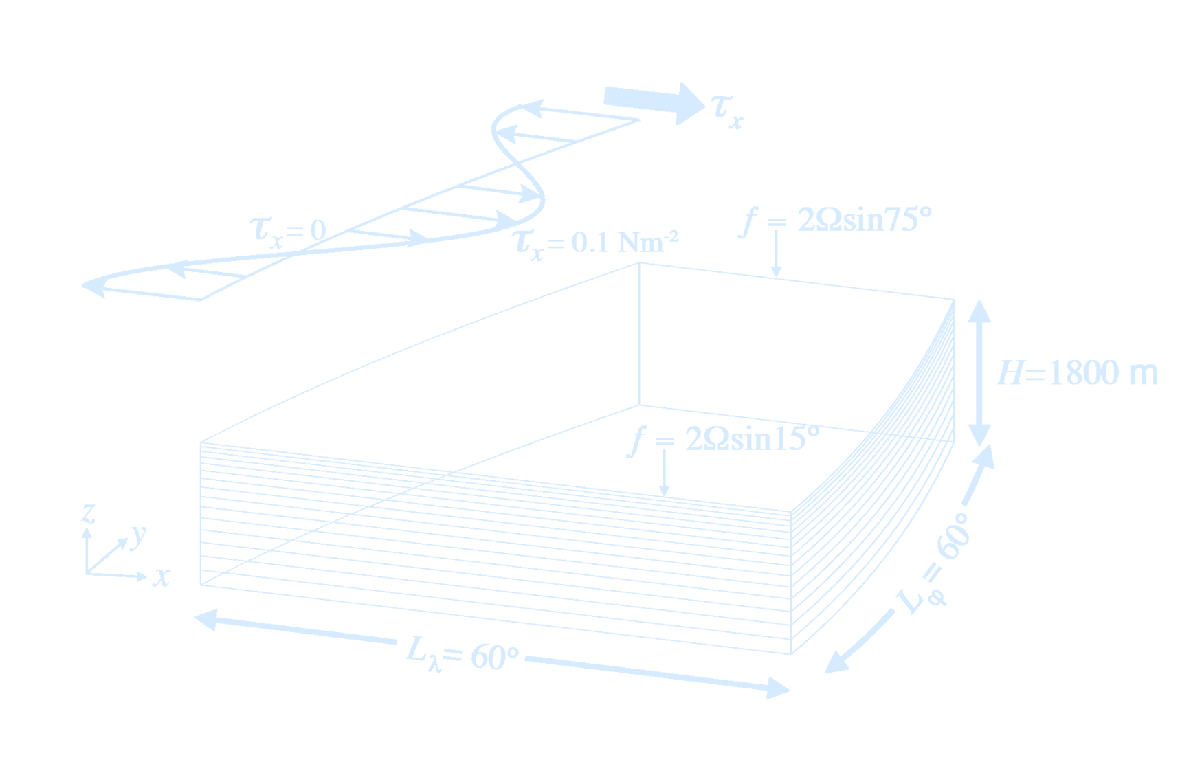
The Coriolis parameter $f$ is defined according to latitude $\varphi$: $$ f(\varphi) = 2\Omega \sin(\varphi) $$ with the rotation rate $\Omega$, set to $$ \Omega = \frac{2\pi}{day} = \frac{2\pi}{86164} \ \text{sec}^{-1} $$ (i.e., corresponding to the standard Earth rotation rate).

Beta-Plane Approximation

The Coriolis parameter $f = 2\Omega \sin\theta$, where $\Omega$ is the angular rotation rate of the Earth and $\theta$ is the latitude. Expand $f$ around $\theta = \theta_o$ using a Taylor series: $$ f = f_o + \left. \frac{\partial f}{\partial \theta} \right|_{\theta_o} \Delta \theta + \left. \frac{\partial^2 f}{\partial \theta^2} \right|_{\theta_o} \frac{\Delta \theta^2}{2} + \dots $$ $$ = 2\Omega \sin \theta_o + 2\Omega \cos \theta_o (\theta - \theta_o) + \mathcal{O}(\Delta \theta^2) $$ $$ = \boxed{f_o + \beta y} $$ where $f_o = 2\Omega \sin \theta_o$ and $\beta = \frac{2\Omega \cos \theta_o}{a}$, as $y = a\Delta \theta$, where $a$ is the radius of the Earth.

The β-plane approximates $f$ as the first two terms of the Taylor Series. The Coriolis parameter changes linearly with latitude.
The f-plane approximates $f$ as the first term of the Taylor Series; $f$ is taken as a constant.

Hydrostatic Approximation

\[0 = - \frac{1}{\rho} p_z + g\] The sum of the pressure gradient and the gravitational force per unit volume must be zero.
The hydrostatic balance is a balance between gravity and the pressure gradient force.

Conservation of Mass

A fundamental law of physics stating that a volume always containing the same atoms and molecules (system) must always contain the same mass. Thus the time rate of change of mass of a system is zero. This law of physics must be revised when matter moves at speeds approaching the speed of light so that mass and energy can be exchanged as per Einstein’s laws of relativity.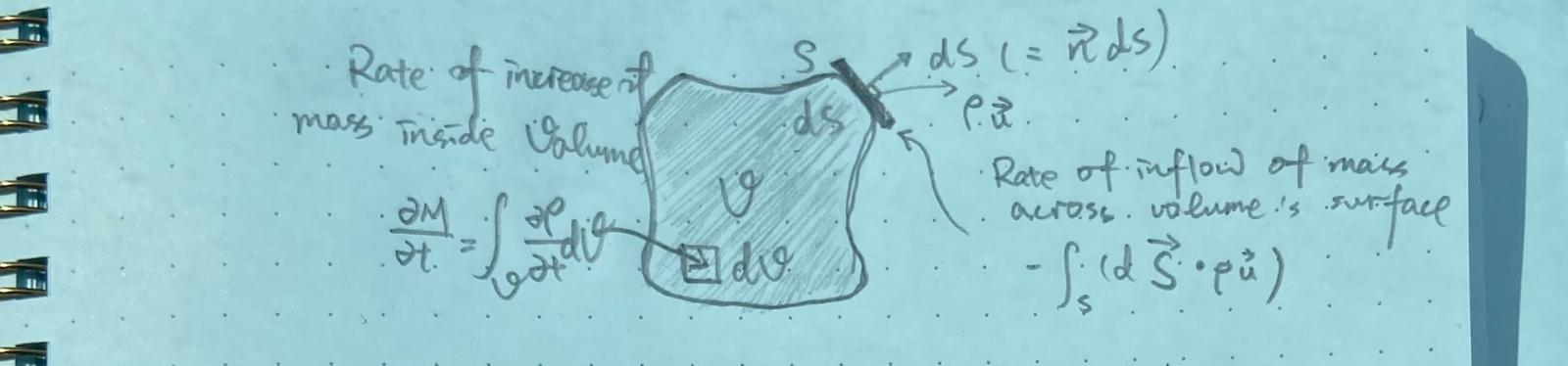 ConservationOfMass

Conservation of Momentum

This is Newton’s second law of motion, a fundamental law of physics stating that the time rate of change of momentum of a fixed mass (system) is balanced by the net sum of all forces applied to the mass.

Continuity Equation

In the absence of sources or sinks of mass within the fluid, the condition of mass conservation is expressed by the continuity equation. In other words, the continuity equation is the mathematical form of conservation of mass applied to a fluid particle in a flow. \[ \frac{\partial \rho}{\partial t} + \nabla \cdot (\rho \mathbf{u}) = 0 \] where $\rho$ is the mass density of the fluid. The equation can be derived by considering a volume $V$ fixed in space, bounded by a surface $S$. If the volume is filled by a fluid with density $\rho$, its mass is $M = \int_V \rho \, dV$
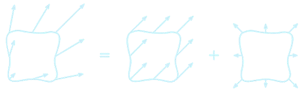
Divergence $\nabla \cdot (\cdots)$ indicates the tendency of a vector field to point outward of a closed surface. When the divergence of velocity $\boxed{\nabla \cdot \mathbf{u}}$ is positive, the fluid is expanding; negative divergence indicates contraction. Imagine a volume of fluid with a complex distribution of $\mathbf{u}$ at its bounding surface, the $\boxed{\nabla \cdot \mathbf{u}}$ calculation will isolate the diverging component (right) from uniform flow (centre).

Equation of State of Seawater

\[ \rho = \rho(\underbrace{T}_{\text{temperature}}, \underbrace{S}_{\text{salinity}}, \underbrace{p}_{\text{pressure}}) \]

Linear Approximation

\[\rho = f(T,S,p) \approx \rho_0(1- \alpha T + \beta S)\] \[ \alpha = \underbrace{\alpha_0}_{\text{reference value}} \left[ 1 + \underbrace{\beta_T (1 + \gamma^* p)(T - T_0)}_{\text{linear thermal expansion}} + \underbrace{\frac{\beta_T^*}{2} (T - T_0)^2}_{\text{nonlinear thermal effect}} - \underbrace{\beta_S (S - S_0)}_{\text{salinity effect}} - \underbrace{\beta_p (p - p_0)}_{\text{pressure effect}} \right] \]

If the equation of state were such that it linked only density and pressure, without introducing another variable, then the equations would be complete; the simplest case of all is a constant density fluid for which the equation of state is just $\rho = \text{constant}$. A fluid for which the density is a function of pressure alone is called a barotropic fluid or a homentropic fluid; otherwise, it is a baroclinic fluid. Equations of state of the form $p = C\rho^\gamma$, where $\gamma$ is a constant, are called polytropic

Barotropic and Baroclinic

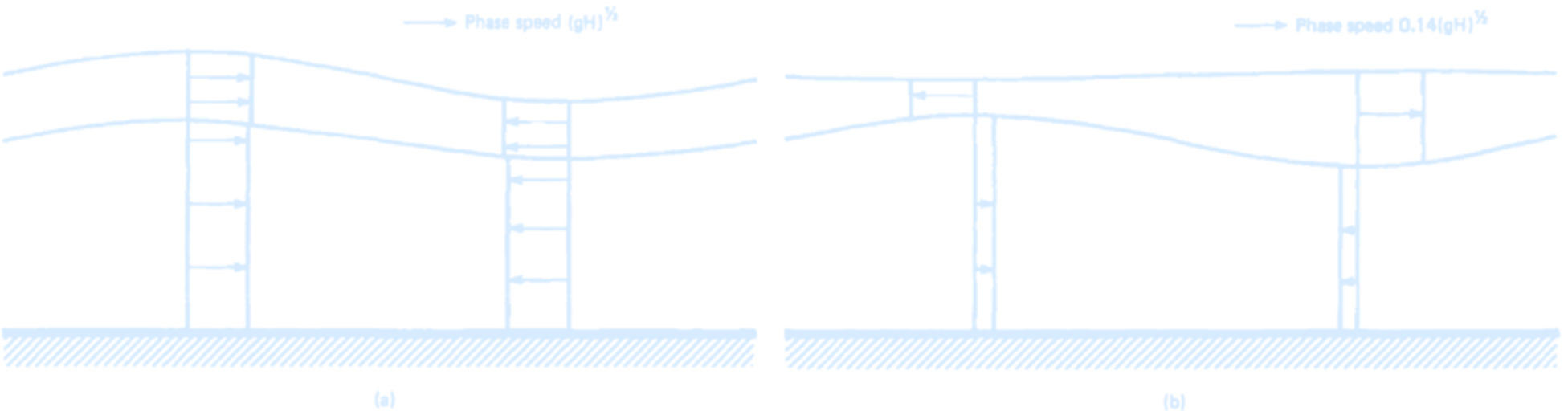
A fluid in which the density depends only on the pressure, $\rho = \rho(p)$, is called a barotropic fluid. A fluid in which the density depends on both temperature and pressure, $\rho = \rho(p, T)$, is called a baroclinic fluid.
In a two-layer ocean

Hydrostatic balance: velocity is depth-independent within any homogeneous layer
For two-layer ocean, two normal modes:
- Layers move together (barotropic)
- Layers move in opposite directions (baroclinic); note vertical average of horizontal velocity is zero.
$N$ layers → $N$ normal modes. Higher modes are progressively slower.

A continuously stratified fluid corresponding to an infinite number of layers, and so there is an infinite set of modes. BaroclinicBarotropic

(Layer configuration in a two-layer system for a barotropic wave (a) and a baroclinic wave (b) propagating from left to right. For the case shown, the lower layer is three times deeper than the upper layer and has density 10% greater. Also shown are the directions of flow at troughs and crests, and the relative velocities of the two layers at these points. Credit: Adrian E. Gill 1982.)

Shear Stress in Fluids

The shear stress of a fluid can be defined as a unit area amount of force acting on the fluid parallel to a very small element of the surface. For the most accurate calculation, the elements should be infinitesimal. The greatest source of stress is the fluid viscosity. Depending upon the medium, shear stress may cause a change in fluid flow between layers.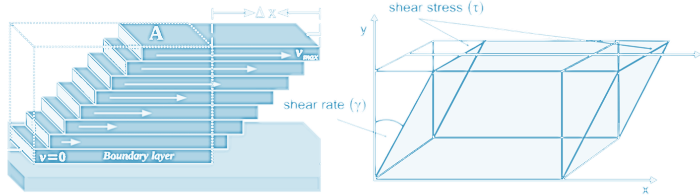 ShearStressShearRate

(Model of fluid flow and relationship between shear stress and shear rate. Credit: Cadence CFD Solutions)

A fluid at rest can not resist shearing forces. Fluids at rest cannot resist a shear stress; in other words, when a shear stress is applied to a fluid at rest, the fluid will not remain at rest, but will move because of the shear stress.
Under the action of such forces it deforms continuously, however small they are. The resistance to the action of shearing forces in a fluid appears only when the fluid is in motion. This implies the principal difference between fluids and solids. For solids the resistance to a shear deformation depends on the deformation itself, that is the shear stress $\tau$ is a function of the shear strain $\gamma$. For fluids the shear stress $\tau$ is a function of the rate of strain $d\gamma/dt$. Shear stress in fluids refers to the force per unit area acting tangentially to the fluid's surface due to its continuous, relative motion.

Viscosity

Shear stress is primarily caused by friction between fluid particles, due to fluid viscosity. The property of a fluid to resist the growth of shear deformation is called viscosity. The form of the relation between shear stress and rate of strain depends on a fluid, and most common fluids obey Newton’s law of viscosity, which states that the shear stress is proportional to the strain rate: $$ \tau = \mu \frac{d\gamma}{dt} $$ Such fluids are called Newtonian fluids. The coefficient of proportionality $\mu$ is known as dynamic viscosity and its value depends on the particular fluid. The ratio of dynamic viscosity to density is called kinematic viscosity $$ \nu = \frac{\mu}{\rho} $$

Steady State Assumption

The continuety equation states that the local increase of density with time must be balanced by a divergence of the mass flux $\rho \mathbf{u}$. This may also be written \[ \frac{d\rho}{dt} + \rho \nabla \cdot \mathbf{u} = 0 \] where \[ \frac{d}{dt} \equiv \frac{\partial}{\partial t} + \mathbf{u} \cdot \nabla \] is the total derivative (often called the substantial derivative) with respect to time of any property following individual fluid elements

Incompressible Navier-Stokes Equations

$$ \overbrace{ \underbrace{\frac{\partial \vec{u}}{\partial t}}_{\text{Local acceleration}} + \underbrace{(\vec{u} \cdot \nabla) \vec{u}}_{\text{Advection}} }^{\text{Material derivative} \frac{D \vec{u}}{D t}} = \underbrace{-\frac{1}{\rho} \nabla P}_{\text{Pressure force}} + \underbrace{g \vec{k}}_{\text{Gravity}} + \underbrace{\nu \nabla^2 \vec{u}}_{\text{Viscous diffusion}} $$ $g \vec{k}$ with typically $ \vec{k} = \begin{pmatrix} 0 \\ 0 \\ 1 \end{pmatrix} $ defines gravity as a vector field acting downward (if you use $-g \vec{k}$, then $\vec{k}$ points upward) The Navier–Stokes equation includes this term: $$ \frac{\partial \vec{u}}{\partial t} + (\vec{u} \cdot \nabla)\vec{u} $$ This expression is the total derivative (also called the material derivative) of velocity $\vec{u}$: $$ \frac{D \vec{u}}{D t} = \frac{\partial \vec{u}}{\partial t} + (\vec{u} \cdot \nabla)\vec{u} $$ Simplification: \[\left(\frac{\partial}{\partial t} + \mathbf{u}\cdot \nabla - \nu \nabla^2\right) \mathbf{u} = - \frac{1}{\rho} \nabla p + f \]

import numpy as np
import matplotlib.pyplot as plt

def incompressible_navier_stokes(u, v, dx, dy, dt, viscosity):
    # Spatial derivatives
    du_dx = np.gradient(u, dx, axis=1)
    du_dy = np.gradient(u, dy, axis=0)
    dv_dx = np.gradient(v, dx, axis=1)
    dv_dy = np.gradient(v, dy, axis=0)
    
    # Laplacians
    laplacian_u = np.gradient(du_dx, dx, axis=1) + np.gradient(du_dy, dy, axis=0)
    laplacian_v = np.gradient(dv_dx, dx, axis=1) + np.gradient(dv_dy, dy, axis=0)
    
    # Update velocities
    u_new = u - dt * (u * du_dx + v * du_dy) + dt * viscosity * laplacian_u
    v_new = v - dt * (u * dv_dx + v * dv_dy) + dt * viscosity * laplacian_v
    
    return u_new, v_new

# Example 
nx, ny = 50, 50
dx, dy = 1.0 / nx, 1.0 / ny
x, y = np.meshgrid(np.linspace(0, 1, nx), np.linspace(0, 1, ny))

u = np.sin(2 * np.pi * x) * np.cos(2 * np.pi * y)
v = -np.cos(2 * np.pi * x) * np.sin(2 * np.pi * y)

dt = 0.001
viscosity = 0.1

# Time-stepping
for _ in range(100):
    u, v = incompressible_navier_stokes(u, v, dx, dy, dt, viscosity)

# Plot
fig, ax = plt.subplots(figsize=(8, 6), dpi = 300)

fig.patch.set_alpha(0.0)
ax.set_facecolor('none')

# Streamplot
ax.streamplot(x, y, u, v, color='#d6ebff')

ax.set_xlabel('x', color='#d6ebff', fontsize=14)
ax.set_ylabel('y', color='#d6ebff', fontsize=14)
ax.tick_params(colors='#d6ebff')
ax.set_title("Incompressible Flow Field", color='#d6ebff', fontsize=16)

# Set frame (spines) color
for spine in ax.spines.values():
    spine.set_edgecolor('#d6ebff')

plt.show()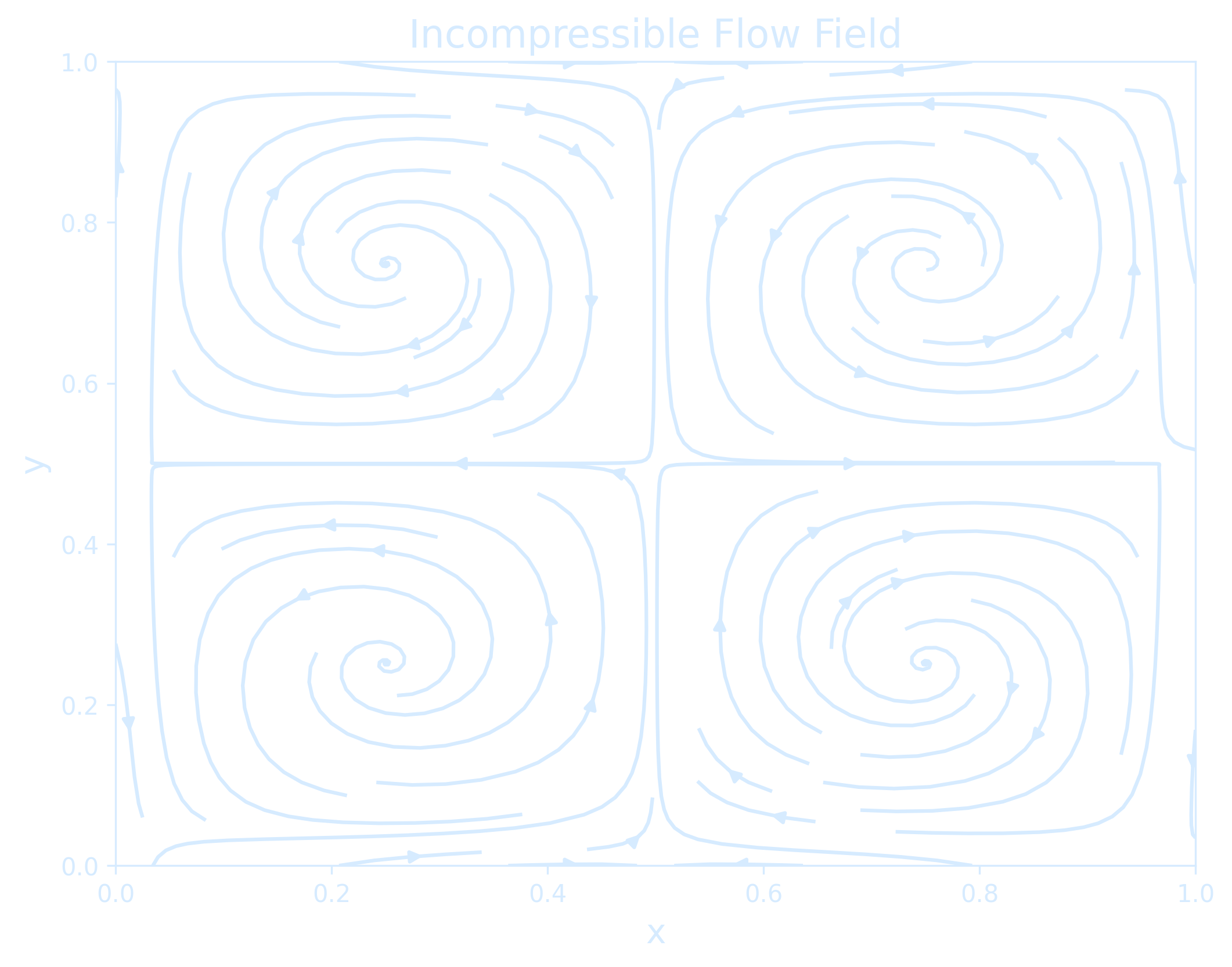

import numpy as np
import matplotlib.pyplot as plt

# Set domain size and grid
nx, ny = 50, 50
dx, dy = 1.0, 1.0
nt = 500
rho = 1.0
mu = 0.1
dt = 0.1

# Initialization
u = np.zeros((nx, ny))
v = np.zeros((nx, ny))
p = np.zeros((nx, ny))

u[24:27, 24:27] = 1.0 # Initial condition: bump in u

def laplacian(f, dx, dy):
    return (
        (f[2:, 1:-1] - 2*f[1:-1, 1:-1] + f[:-2, 1:-1]) / dx**2 +
        (f[1:-1, 2:] - 2*f[1:-1, 1:-1] + f[1:-1, :-2]) / dy**2
    )

def pressure_poisson(p, u, v, dx, dy, rho, dt):
    b = rho * ((u[2:,1:-1] - u[:-2,1:-1]) / (2*dx) +
               (v[1:-1,2:] - v[1:-1,:-2]) / (2*dy)) / dt
    for _ in range(50):  # Iterative solver
        p[1:-1, 1:-1] = 0.25 * (
            p[2:, 1:-1] + p[:-2, 1:-1] +
            p[1:-1, 2:] + p[1:-1, :-2] -
            b * dx**2
        )
    return p

def solve_coupled(u, v, p, mu, dx, dy, dt, rho, nt):
    for _ in range(nt):
        u_old = u.copy()
        v_old = v.copy()

        # Pressure Poisson solve (right-hand side: velocity divergence)
        p = pressure_poisson(p, u_old, v_old, dx, dy, rho, dt)

        # Update u using pressure gradient and diffusion
        u[1:-1, 1:-1] = u_old[1:-1, 1:-1] - dt / rho * (p[2:, 1:-1] - p[:-2, 1:-1]) / (2 * dx) + \
                        mu * dt * laplacian(u_old, dx, dy)

        # Update v using pressure gradient and diffusion
        v[1:-1, 1:-1] = v_old[1:-1, 1:-1] - dt / rho * (p[1:-1, 2:] - p[1:-1, :-2]) / (2 * dy) + \
                        mu * dt * laplacian(v_old, dx, dy)

    return u, v, p

# Solve the equations
u, v, p = solve_coupled(u, v, p, mu, dx, dy, dt, rho, nt)

plt.figure(figsize=(15, 5), dpi=300)

plt.subplot(1, 3, 1)
plt.title('Velocity field (u)', color='#d6ebff')
plt.imshow(u.T, origin='lower', cmap='coolwarm')
plt.colorbar(label='u')
plt.axis('off')

plt.subplot(1, 3, 2)
plt.title('Velocity field (v)', color='#d6ebff')
plt.imshow(v.T, origin='lower', cmap='coolwarm')
plt.colorbar(label='v')
plt.axis('off')

plt.subplot(1, 3, 3)
plt.title('Pressure field', color='#d6ebff')
plt.imshow(p.T, origin='lower', cmap='coolwarm')
plt.colorbar(label='p')
plt.axis('off')

plt.tight_layout()
plt.show()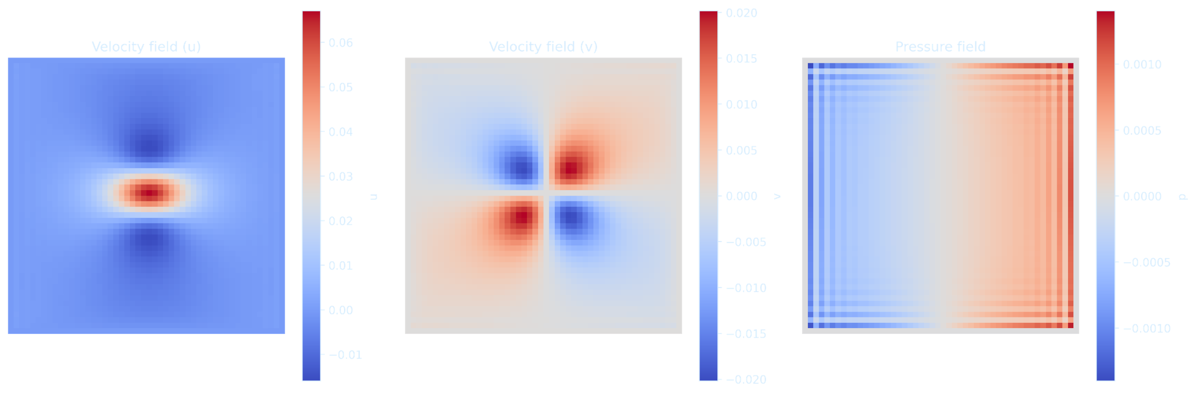

Bonus: Navier-Lamé Equation

$$ \overbrace{ \underbrace{\rho}_{\text{Density}} \, \underbrace{\frac{\partial^2 \mathbf{u}}{\partial t^2}}_{\text{Acceleration}} }^{\vec{ma}} = \overbrace{ \underbrace{\mathbf{f}}_{\text{Body force}} + \underbrace{(\lambda + \mu)}_{\substack{\text{Lamé parameters $\lambda, \mu$} \\ \text{(material constants governs compressibility effects)}}} \, \underbrace{\nabla (\nabla \cdot \mathbf{u})}_{\substack{\text{gradient of} \\ \text{the divergence}}} + \underbrace{\mu \nabla^2 \mathbf{u}}_{\text{shear (Laplacian) term}} }^{\text{Total force } \vec{F}_{\text{total}} \text{ (body + elastic)}} $$ This equation is one of the most fundamental equations in Earthquake Seismology, and the vast majority of content in Earthquake Seismology derived from it.

Bonus: How Do Airplanes Fly?

Hydrostatic Ocean on a Rotating Sphere

Zonal (East–West) Momentum Equation: $$ \frac{\partial u}{\partial t} + \vec{u} \cdot \nabla u - fv = -\frac{1}{\rho_0} \frac{\partial p}{\partial x} + \nu \nabla^2 u + \underbrace{F^x}_{{\substack{\text{External forcing} \\ \text{in the x-direction} \\ \text{(typically wind stress } \tau^x\text{)}}}} $$ Meridional (North–South) Momentum Equation: $$ \frac{\partial v}{\partial t} + \vec{u} \cdot \nabla v + fu = -\frac{1}{\rho_0} \frac{\partial p}{\partial y} + \nu \nabla^2 v + \underbrace{F^y}_{{\substack{\text{External forcing} \\ \text{in the y-direction} \\ \text{(typically wind stress } \tau^y\text{)}}}} $$ Hydrostatic Balance (Vertical): $$ \frac{\partial p}{\partial z} = -\rho g $$ Continuity (Incompressibility): $$ \nabla \cdot \vec{u} = \frac{\partial u}{\partial x} + \frac{\partial v}{\partial y} + \frac{\partial w}{\partial z} = 0 $$

Ekman Transport

In the Northern Hemisphere, the net volume transport direction of seawater is 90° to the right (northeastward) of the wind direction. This transport of water masses is known as Ekman Transport, and the spiral pattern of current vectors changing with increasing depth is called the Ekman Spiral.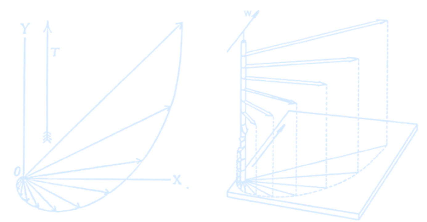 EkmanSpiral

(Credit: Ekman, V.W.(1905) On the Influence of the Earth's Rotation on Ocean-Currents. Arkiv För Matematic, Astronomi och Fysik, Bd 2, N:o 11, 1-53.)

[Q] What does an Ekman spiral look like at the surface? Is it strong enough to disturb ships?
[A] The Ekman spiral creates different layers of surface water that move in slightly different directions at slightly different speeds. It is too weak to create eddies or whirlpools (vortexes) at the surface and so presents no danger to ships. In fact, the Ekman spiral is unnoticeable at the surface. It can be observed, however, by lowering oceanographic equipment over the side of a vessel. At various depths, the equipment can be observed to drift at various angles from the wind direction according to the Ekman spiral.

Ekman flow in NH is 90º to the right of the wind stress
Cyclonic wind (around low presure) forces divergence in water, and upwelling
Anticyclonic wind (around high pressure) forces convergence and downwelling

Use the files ERA5_LowRes_MonthlyAvg_uvslp.nc and ERA5_LowRes_Invariant.nc as examples. The first step in calculating the Ekman currents is obtaining wind stress from the wind velocity.

import numpy as np
import xarray as xr
import matplotlib.pyplot as plt
import cartopy.crs as ccrs
import cartopy.feature as cfeature
import os
import imageio

output_dir = 'windstress_gif_frames'
gif_path = 'windstress_animation.gif'
os.makedirs(output_dir, exist_ok=True)

# Load data
ds = xr.open_dataset('ERA5_LowRes_MonthlyAvg_uvslp.nc')

# Constants
rho_air = 1.225
cd = 1.5e-3
R = 6371000
dpi = 300
tick_color = '#d6ebff'
step = 5  # vector density

# Compute wind stress
u10 = ds['u10']
v10 = ds['v10']
ws = np.sqrt(u10**2 + v10**2)
tau_x = rho_air * cd * ws * u10
tau_y = rho_air * cd * ws * v10
tau = np.sqrt(tau_x**2 + tau_y**2)

lon = ds.longitude
lat = ds.latitude

# Use a fixed vmin/vmax across all frames for consistent colorbar
tau_vmin = float(tau.min().values)
tau_vmax = float(tau.max().values)

image_paths = []


for month_index in range(len(ds['month'])):
    tau_plot = tau.isel(month=month_index)
    tau_x_plot = tau_x.isel(month=month_index)
    tau_y_plot = tau_y.isel(month=month_index)

    fig = plt.figure(figsize=(10, 5), dpi=dpi)
    ax = fig.add_subplot(1, 1, 1, projection=ccrs.PlateCarree())

    # Plot tau manually to allow control over colorbar
    mesh = ax.pcolormesh(
        lon, lat, tau_plot,
        cmap='Greens',
        vmin=tau_vmin, vmax=tau_vmax,
        transform=ccrs.PlateCarree()
    )

    # Add quiver
    ax.quiver(
        lon[::step], lat[::step],
        tau_x_plot.values[::step, ::step],
        tau_y_plot.values[::step, ::step],
        transform=ccrs.PlateCarree(), scale=700, color=tick_color
    )


    ax.coastlines()
    ax.add_feature(cfeature.BORDERS, linewidth=0.5, edgecolor=tick_color)
    gl = ax.gridlines(draw_labels=True, color=tick_color, linestyle='--', linewidth=0.3)
    gl.xlabel_style = {'color': tick_color}
    gl.ylabel_style = {'color': tick_color}

    # Colorbar
    cbar = fig.colorbar(mesh, ax=ax, orientation='vertical', pad=0.02, shrink=0.8)
    cbar.set_label("Wind Stress (N/m²)", color=tick_color)
    cbar.outline.set_edgecolor(tick_color)
    cbar.ax.yaxis.set_tick_params(color=tick_color)
    plt.setp(cbar.ax.yaxis.get_ticklabels(), color=tick_color)

    # Overlay month label (bottom left corner)
    ax.text(
        0.02, 0.02, f"Month {month_index}",
        transform=ax.transAxes,
        fontsize=14, color=tick_color,
        ha='left', va='bottom',
        bbox=dict(facecolor='white', edgecolor=tick_color, alpha=0.5, boxstyle='round,pad=0.3')
    )

    # Save frame
    frame_path = os.path.join(output_dir, f'windstress_frame_{month_index:02d}.png')
    plt.tight_layout()
    plt.savefig(frame_path, dpi=dpi, bbox_inches='tight', facecolor='none')
    image_paths.append(frame_path)
    plt.close()

# Create GIF with infinite loop
with imageio.get_writer(gif_path, mode='I', duration=3, loop=0) as writer: # duration: x seconds per frame
    for path in image_paths:
        image = imageio.imread(path)
        writer.append_data(image)

print(f"GIF created at: {gif_path}")

The transport of water integrated over the Ekman layer is: \[ M_{ek} = \frac{\tau_{wind} \times \hat{z}}{f} \] From the zonal and meridional components we can calculate the Ekman transport using: \[ M_x = \frac{\tau_y}{f} \] \[ M_y = -\frac{\tau_x}{f} \] Where $M_x$ is the zonal Ekman transport, $M_y$ is the meridional Ekman transport, and $f$ is the Coriolis parameter depends on the latitude $\theta$: \[ f = 2\Omega \sin(\theta) \] Where $\Omega$ is the angular velocity of the Earth

# Compute Coriolis parameter f (on 1D latitude, then broadcast to 2D)
lat = ds.latitude
f = 2 * 7.2921150e-5 * np.sin(np.deg2rad(lat))  # Coriolis at each latitude
f = f.where((np.abs(lat) > 3) & (np.abs(lat) < 87))  # mask equator & poles

# Broadcast f to match tau shape
f2d = f.broadcast_like(tau_x_plot)

# Compute Ekman transport (m²/s)
mek_x = tau_y_plot / f2d
mek_y = -tau_x_plot / f2d

# Create 2D meshgrid of lat/lon in radians
lon2d, lat2d = np.meshgrid(ds.longitude, ds.latitude)
lat2d_rad = np.deg2rad(lat2d)
lon2d_rad = np.deg2rad(lon2d)

# Grid spacing in meters 
dy = R * np.gradient(lat2d_rad, axis=0)  # dφ
dx = R * np.cos(lat2d_rad) * np.gradient(lon2d_rad, axis=1)  # dλ * cos(φ)

# Compute gradients of transport (divergence)
d_mek_x_dx = np.gradient(mek_x, axis=1) / dx
d_mek_y_dy = np.gradient(mek_y, axis=0) / dy

# Compute Ekman pumping (m/s → m/year)
wek = (d_mek_x_dx + d_mek_y_dy) / rho_water
wek = wek * 60 * 60 * 24 * 365  # m/year

# Convert to xarray for plotting
wek_da = xr.DataArray(
    wek,
    coords={"latitude": ds.latitude, "longitude": ds.longitude},
    dims=["latitude", "longitude"]
)

tick_color = '#d6ebff'  
fig, ax = plt.subplots(figsize=(13, 5), subplot_kw={'projection': ccrs.PlateCarree()})

# Plot the data
plot = wek_da.plot(
    ax=ax,
    transform=ccrs.PlateCarree(),
    cmap='RdBu_r',
    vmin=-50,
    vmax=50,
    cbar_kwargs={'label': 'Ekman Pumping (m/year)'}
)

ax.set_title("Ekman Pumping (Vertical Velocity from Wind Stress)", fontsize=14, color=tick_color)
ax.coastlines()
ax.add_feature(cfeature.BORDERS, linewidth=0.5, edgecolor=tick_color)
# Gridlines
gl = ax.gridlines(draw_labels=True, color=tick_color, linestyle='--', linewidth=0.3)
gl.xlabel_style = {'color': tick_color}
gl.ylabel_style = {'color': tick_color}

cbar = plot.colorbar
cbar.outline.set_edgecolor(tick_color)
cbar.ax.yaxis.set_tick_params(color=tick_color)
plt.setp(cbar.ax.yaxis.get_ticklabels(), color=tick_color)
cbar.set_label("Ekman Pumping (m/year)", color=tick_color)

#plt.savefig('Lecture2_EkmanPumping.png', dpi=300, bbox_inches='tight', facecolor='none')
plt.show()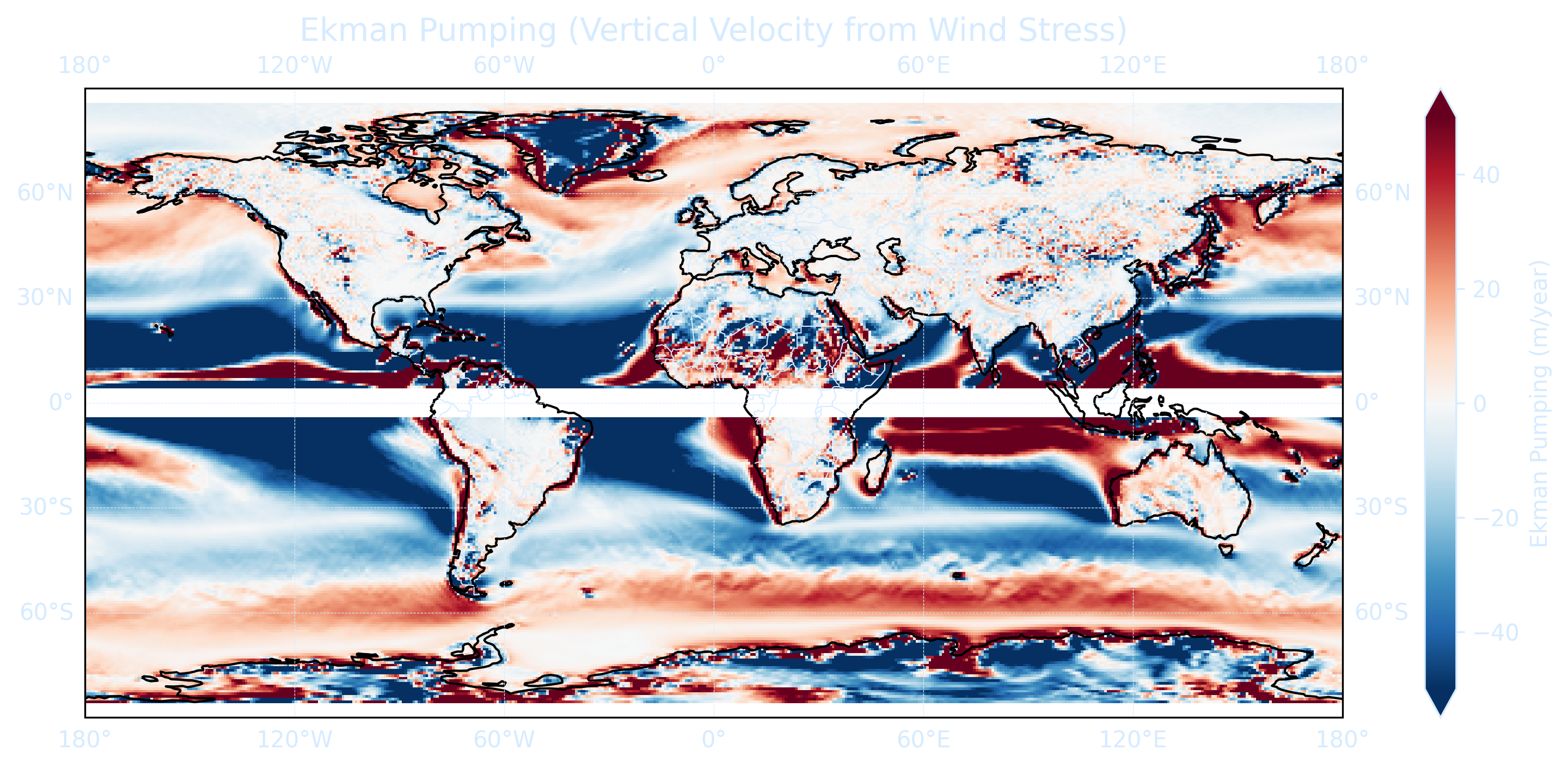

One problem with the calculation of Ekman transport is that it tends to infinity close to the equator. Now try to make a combined streamline plot and mask a band of 3 degrees around the equator.

import numpy as np
import xarray as xr
import matplotlib.pyplot as plt
import cartopy.crs as ccrs
import cartopy.feature as cf
import matplotlib.ticker as mticker
from cartopy.mpl.ticker import LongitudeFormatter, LatitudeFormatter
import matplotlib.cm as cm

ds = xr.open_dataset('ERA5_LowRes_MonthlyAvg_uvslp.nc')
month_index = 0  # Choose a month to visualize

# Constants
rho_air = 1.225
cd = 1.5e-3
rho_water = 1000
R = 6371000  # Earth radius in meters
tick_color = '#d6ebff'  # consistent theme

# Extract wind components
u10 = ds['u10'].isel(month=month_index)
v10 = ds['v10'].isel(month=month_index)
ws = np.sqrt(u10**2 + v10**2)
tau_x = rho_air * cd * ws * u10
tau_y = rho_air * cd * ws * v10
lat = ds.latitude
lon = ds.longitude

# Coriolis parameter (masked at equator/poles)
f = 2 * 7.2921150e-5 * np.sin(np.deg2rad(lat))
f2d = f.broadcast_like(tau_x)

# Ekman transport
Mx = tau_y / f2d
My = -tau_x / f2d

# Apply equatorial mask
mask = np.abs(lat) < 3
mask_np = np.broadcast_to(mask.values[:, np.newaxis], Mx.shape)
Mx_np = np.ma.masked_where(mask_np, Mx.values)
My_np = np.ma.masked_where(mask_np, My.values)
Mmag_np = np.sqrt(Mx_np**2 + My_np**2)

# Meshgrid for plotting
lon2d, lat2d = np.meshgrid(lon, lat)

# Plot
fig = plt.figure(figsize=(15, 5), dpi=300)
ax = plt.axes(projection=ccrs.PlateCarree(central_longitude=180))
ax.set_extent([120, 300, -60, 60], crs=ccrs.PlateCarree())
ax.coastlines()
ax.add_feature(cf.BORDERS, linewidth=0.5, edgecolor=tick_color)

# Gridlines styled
gl = ax.gridlines(draw_labels=True, color=tick_color, linestyle='--', linewidth=0.3)
gl.xlabels_top = False
gl.ylabels_right = False
gl.xlabel_style = {'color': tick_color}
gl.ylabel_style = {'color': tick_color}
gl.xlocator = mticker.FixedLocator([120, 150, 180, -150, -120, -90, -60])
gl.ylocator = mticker.FixedLocator([-60, -40, -20, 0, 20, 40, 60])
gl.xformatter = LongitudeFormatter()
gl.yformatter = LatitudeFormatter()

# Streamplot of Ekman transport
strm = ax.streamplot(
    lon2d, lat2d, Mx_np, My_np,
    transform=ccrs.PlateCarree(),
    color=Mmag_np,
    density=5,
    linewidth=2,
    cmap=cm.jet
)

ax.set_title("Ekman Transport (from Wind Stress)", fontsize=14, color=tick_color, pad=10)

cbar = fig.colorbar(strm.lines, ax=ax, orientation='vertical', pad=0.02, shrink=0.8)
cbar.set_label("Transport Magnitude (m²/s)", color=tick_color)
cbar.outline.set_edgecolor(tick_color)
cbar.ax.yaxis.set_tick_params(color=tick_color)
plt.setp(cbar.ax.yaxis.get_ticklabels(), color=tick_color)

plt.savefig("ekman_transport_streamplot.png", dpi=300, bbox_inches='tight', facecolor='none')
plt.show()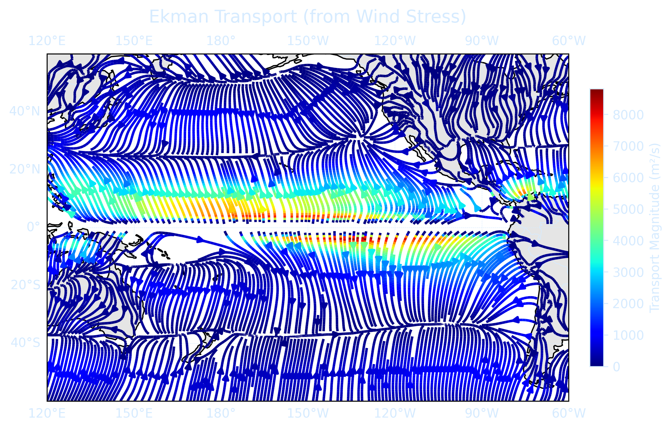

Sverdrup Relation

\[ V = \frac{1}{\rho_0 \beta} \nabla \times \tau \] $V$ is the meridional (north–south) transport, $\rho_0 \approx 1024 \, \text{kg m}^{-3}$ the density of sea water, $\beta$ the Rossby parameter, and $\tau$ the surface wind stress. We study the connection of the Sverdrup relation to the barotropic streamfunction $\Psi$, for which \[ \frac{\partial \Psi}{\partial y} = -U, \quad \frac{\partial \Psi}{\partial x} = V \]

Depth integral over Sverdrup Relation
The Sverdrup balance describes the relationship between the curl of the wind stress $\tau$ and the vertical integral of the horizontal velocity V in the ocean
Illustrates how wind stress drives large-scale ocean circulation patterns, such as gyres, by inducing a circulation balanced by the Coriolis force

Thermal Wind

In the presence of a horizontal gradient of density, the geostrophic velocity develops a vertical shear. This can be shown from the geostrophic and hydrostatic balances by differentiating both parts of geostrophic balance with respect to $z$ and then using $ \frac{dp}{dz} = -\rho g $ to eliminate $p$ from both equations: $$ \frac{\partial v}{\partial z} = -\frac{g}{\rho_0 f} \frac{\partial \rho}{\partial x} \quad \text{and} \quad \frac{\partial u}{\partial z} = \frac{g}{\rho_0 f} \frac{\partial \rho}{\partial y} $$ Meteorologists call these the thermal wind equations because they give the vertical variation of wind from measurements of horizontal temperature (and pressure) gradients.

Wind Driven Gyres

The near-surface circulation and density structure are dominated by the wind-driven circulation. The vertically integrated wind-driven gyres are qualitatively described by the Sverdrup relation. \[ U_x + V_y = 0 \] \[ U = \frac{-1}{\beta\rho_0} \int_x^{x_e} (\text{curl} \tau)_y \text{d}x \]

Assume $\tau^y = 0$ and $\tau^x_x = 0$

\[ U = \frac{1}{\beta \rho_0} \tau^x_{yy} \Delta x \]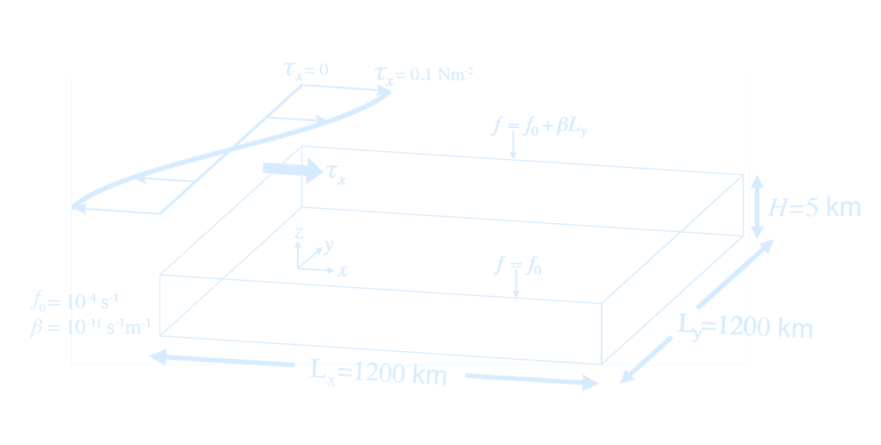 BarotropicGyreNumericalExperiment

$ \text{I} \quad -fv = -\frac{1}{\rho_0} p_x + \frac{1}{\rho_0} \tau^x_z $
$ \text{II} \quad fu = -\frac{1}{\rho_0} p_y + \frac{1}{\rho_0} \tau^y_z $
$ \text{III} \quad 0 = -\frac{1}{\rho} p_z + g $
$ \text{IV} \quad u_x + v_y + w_z = 0 \quad \text{(continuity equation)} $
What were our assumptions/approximations that got us here? $(II)_x - (I)_y$, combine with continuity equation (IV): \[ \beta v = f w_z + \frac{1}{\rho_0} \frac{\delta}{\delta z} \text{curl} \, \vec{\tau} \quad \text{no friction below the mixed layer, so} \] At the ocean top and bottom $w = 0$, so a depth integral yields: \[ \vec{V}_S = \frac{1}{\beta \rho_0} \text{curl} \, \vec{\tau} \quad \boxed{\textbf{!!! The Sverdrup Balance!}} \] What about $U$, the zonal transport? At the ocean top and bottom $w = 0$, so a depth integral of IV yields: $$ U_x + V_y = 0 $$ which, combined with $\vec{V}_S = \frac{1}{\beta \rho_0} \text{curl} \, \vec{\tau}$, yields: $$ U = -\frac{1}{\beta \rho_0} \int_x^{x_e} (\text{curl} \, \vec{\tau})_y \, dx $$ Let’s assume $\tau^y = 0$ and $\tau^x_x = 0$, so: $$ U = \frac{1}{\beta \rho_0} \tau^x_{yy} \, \Delta x $$

The flow is proportional to the curvature of the zonal wind stress, not the wind itself.

Key Equation: $$ \boxed{ \beta V = f w_E } $$ Where:

$\beta = \frac{\partial f}{\partial y}$
$V$: vertically integrated meridional velocity $\int v \, dz$
$w_E$: vertical velocity at base of Ekman layer (Ekman pumping/suction)

Using the Ekman pumping velocity from wind stress: $$ w_E = \frac{1}{\rho_0 f} \, \nabla \cdot \boldsymbol{\tau} = \frac{1}{\rho_0 f} \, \text{curl}_z(\boldsymbol{\tau}) $$ Final Sverdrup Transport (Depth-Integrated Form): $$ \boxed{ V_s = \frac{1}{\beta \rho_0} \, \text{curl}_z(\boldsymbol{\tau}) } $$ This is the classic Sverdrup balance, showing how the wind stress curl determines large-scale meridional transport in the ocean interior.

The Oceanic Mixed Layer and Thermocline

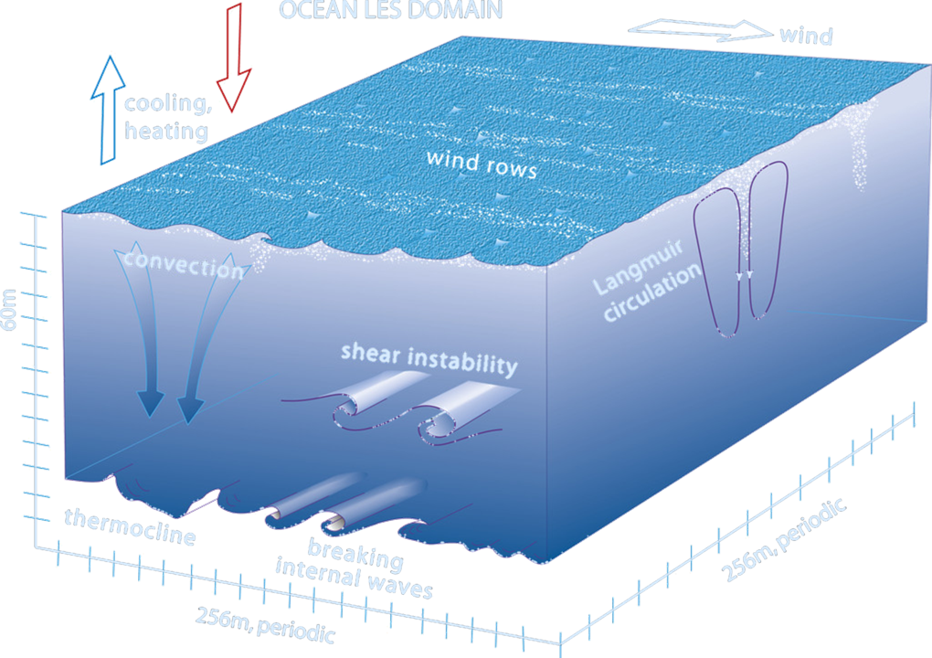
The stratification of the ocean is decidedly nonuniform in the vertical. The density is almost uniform in a layer at the top of the ocean about 50–100 m deep known as the mixed layer. The density then increases fairly rapidly over a region 500–1000 m deep known as the pycnocline, and is then fairly uniform in the abyss. The weak stratification in the abyss and in the mixed layer will inhibit the propagation of internal waves generated in the thermocline.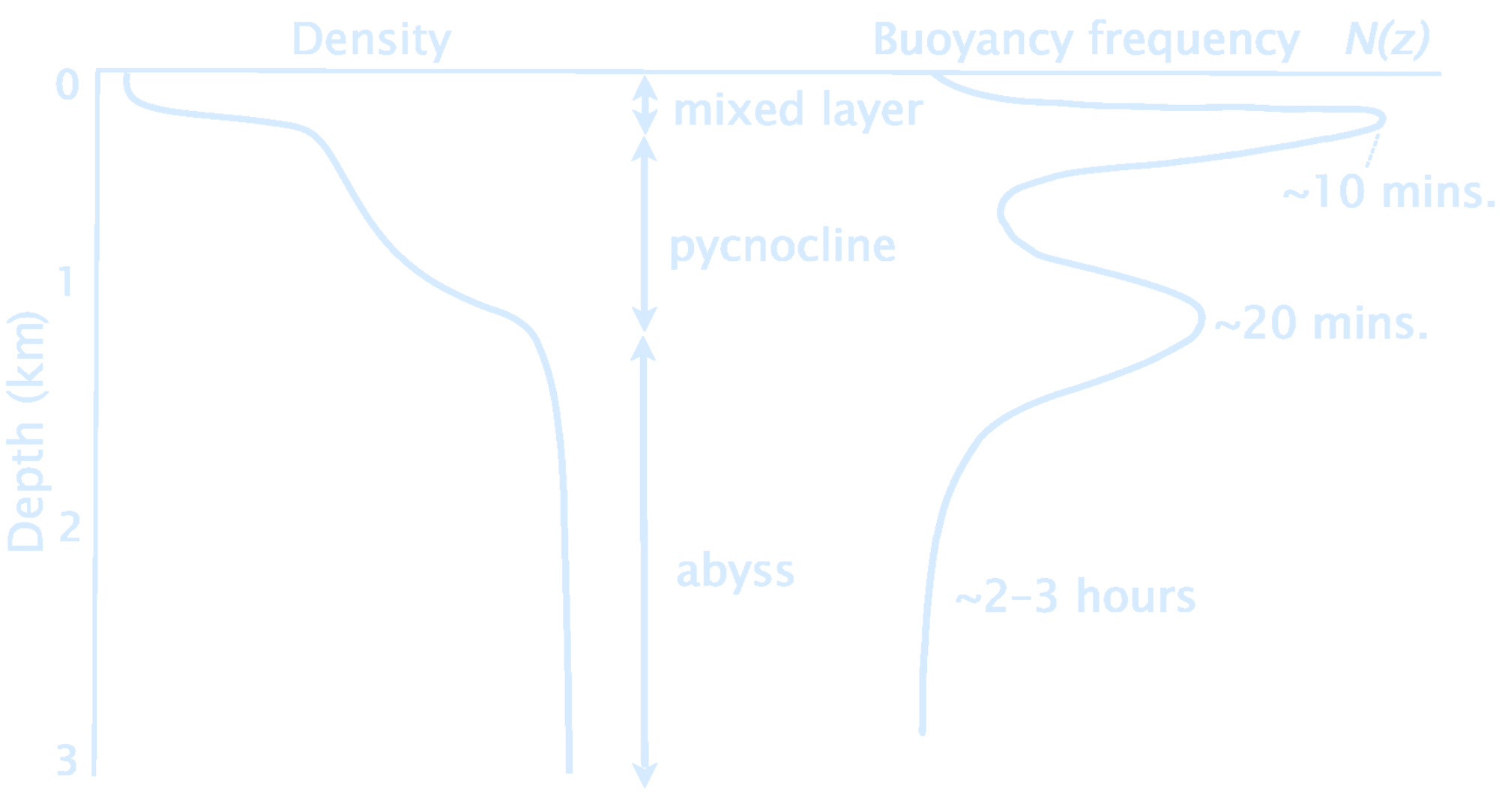 OceanDensityProfile

(Sketch of an ocean density profile, left, and buoyancy frequency, right, labelled with the approximate period. The pycnocline is sandwiched between two weakly stratified regions. The double peak in the buoyancy frequency is exaggerated, but the pycnocline is generally the region of highest frequency internal waves. Credit: G. Vallis, 2017.)

Wind blowing on the ocean stirs the upper layers, leading to a thin mixed layer at the sea surface having constant temperature and salinity from the surface down to a depth where the values differ from those at the surface. The depth and temperature of the mixed layer varies from day to day and from season to season in response to two processes:

Heat fluxes through the surface heat and cool the surface waters. Changes in temperature change the density contrast between the mixed layer and deeper waters. The greater the contrast, the more work is needed to mix the layer downward and visa versa.
Turbulence in the mixed layer mixes heat downward. The turbulence depends on the wind speed and on the intensity of breaking waves. Turbulence mixes water in the layer, and it mixes the water in the layer with water in the thermocline.

The mid-latitude mixed layer is thinnest in late summer when winds are weak, and sunlight warms the surface layer. At times, the heating is so strong, and the winds so weak, that the layer is only a few meters thick. In fall, the first storms of the season mix the heat down into the ocean thickening the mixed layer, but little heat is lost. In winter, heat is lost, and the mixed layer continues to thicken, becoming thickest in late winter. In spring, winds weaken, sunlight increases, and a new mixed layer forms. Below the mixed layer, water temperature decreases rapidly with depth except at high latitudes. The range of depths where the rate of change, the gradient of temperature, is large is called the thermocline. Because density is closely related to temperature, the thermocline also tends to be the layer where density gradient is greatest, the pycnocline.

The mixed layer tends to be saltier than the thermocline between $10^\circ$ and $40^\circ$ latitude, where evaporation exceeds precipitation.
At high latitudes, the mixed layer is fresher because rain and melting ice reduce salinity.
In some tropical regions, such as the warm pool in the western tropical Pacific, rain also produces a thin, fresher mixed layer.

(Schematic of the upper-ocean showing surface forcing and subsurface mixing processes. Credit: Hoecker-Martínez, Smyth, and Skyllingstad, 2016.)

Next: Lecture 3 – Origin of Carbon and Water on Earth