Lecture 4 – The Gulfstream

Geostrophy

Large-scale flow in the ocean and the atmosphere is characterized by an approximate balance in the vertical direction between the pressure gradient and gravity (hydrostatic balance), and in the horizontal direction between the pressure gradient and the Coriolis force (geostrophic balance). The Coriolis force in the momentum equations leads to the possibility of new balances, in particular, a balance between the Coriolis force and the pressure gradient force (geostrophic balance). There is an acceleration from high to low pressure, as would happen without any influence of rotation.
acceleration = pressure gradient force $$ \frac{\partial u}{\partial t} = -\frac{1}{\rho_0} \frac{\partial p}{\partial x} $$ Over time, as the velocity $u$ increases, the Coriolis force becomes important. If the pressure gradient persists over a time longer than the inertial period, $T = \frac{2\pi}{f}$, the water parcel will be deflected (to the right in the Northern Hemisphere), until the Coriolis force exactly balances the pressure gradient force. The parcel will then experience no further accelerations (at least in our rotating reference frame). Remember that: $$ f = 2\Omega \sin \theta \quad \text{where} \quad \Omega = \frac{2\pi}{24 \text{ hours}} = 7.292 \times 10^{-5} \, \text{s}^{-1} $$ and $\theta$ is latitude. Then we have Geostrophy: $$ \boxed{fu = -\frac{1}{\rho_0} \frac{\partial p}{\partial y}} \quad \left( F_c = -F_p \right) $$ Geostrophy also holds for the other velocity component $v$: $$ \boxed{fv = \frac{1}{\rho_0} \frac{\partial p}{\partial x}} $$ The signs for the component equations $fu = -\frac{1}{\rho_0} \frac{\partial p}{\partial y}$ and $fv = \frac{1}{\rho_0} \frac{\partial p}{\partial x}$ are because of the high pressure is on the right when looking downstream in the northern hemisphere (and on the left in the southern hemisphere, where $f$ is negative).
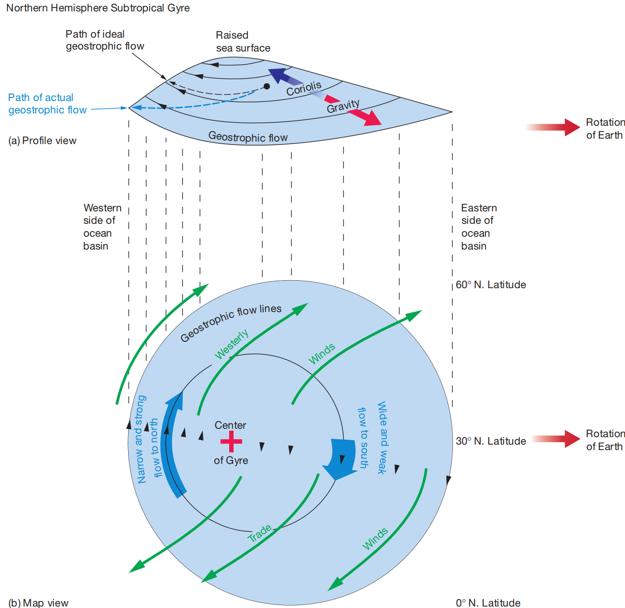
The horizontal movement of surface water arising from a balance between the pressure gradient force and the Coriolis force is known as geostrophic flow. Viewed from above, geostrophic flow in a subtropical gyre is clockwise in the Northern Hemisphere and counterclockwise in the Southern Hemisphere. Geostrophic flow is the balance between Coriolis effects causing currents to form a bulge of water in the center of ocean gyres and gravity currents also affected by the Coriolis effect. The geostropic flow is shown as concentric rings around the bulge in the figure below:

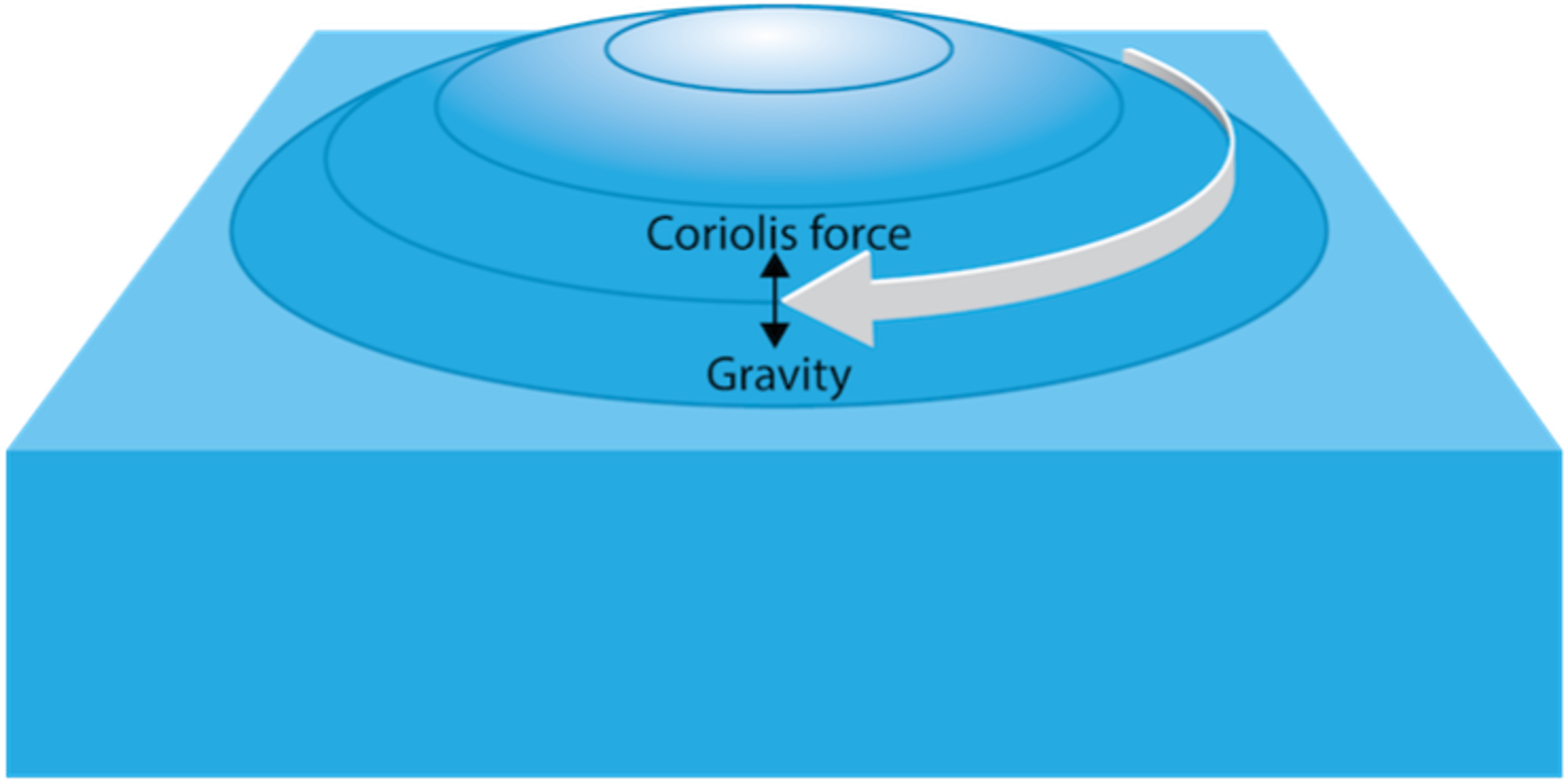
• Convergence of Ekman flow raises sea surface
• Rotating “dome” results

Ocean Currents

In the process of ocean current classification, there exist various standards, including the direction, temperature, origin, and location of ocean currents.

Classification Factor	Subcategories	Detailed Classification Criteria
Temperature	Warm current, Cold current	Classified by comparing the temperature of ocean currents with surrounding waters. Currents warmer than surroundings are warm currents; colder ones are cold currents. Currents flowing from low to high latitudes are typically warm currents, and vice versa.
Driving Mechanism	Wind-driven current (Drift current), Density current, Compensating current	Ocean currents are mainly driven by two forces: one is wind stress on the sea surface, and the other is density differences in seawater.
Vertical Transport Direction	Upwelling, Downwelling	Classified based on vertical flow: movement from deeper waters to the surface is upwelling, and the reverse is downwelling.
Geographic Region	Equatorial current, Shelf current, Eastern/Western boundary current, Coastal current	Different regions have different sunlight, wind, and precipitation conditions, which affect ocean properties and lead to different regional current characteristics.
Equilibrium State	Geostrophic current, Inertial current, etc.	Classified by the balance of forces acting on ocean currents and the number of force components.

The table above shows several commonly used classification standards and examples. In practical, a frequently encountered type of ocean current is the Circulation. Circulation refers to a spiral flow pattern within a curved current, where the flow forms a circular motion when projected onto a cross-section.

Boundary Layer

A boundary layer is a thin layer of viscous fluid in the immediate vicinity of a solid surface, which is also known as a frictional layer. The no-slip condition at the interface between the fluid and the solid surface creates a sharp velocity gradient normal to the wall. Therefore, viscous forces cannot be disregarded inside a boundary layer. Outside the thin boundary region, the viscous forces are usually ignored due to the small velocity gradient.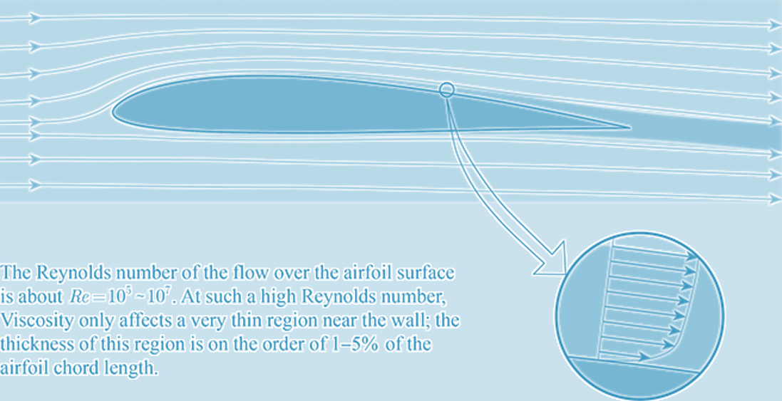 Prandtl’s breakthrough was built on the fact that, in general flows, viscosity is only significant within the very thin near-wall layer called the boundary layer, outside of which the flow (generally called mainstream) is essentially inviscid.

Western Boundary Currents

\( u_t + \vec{u} \cdot \nabla u - fv = -\frac{1}{\rho_0}p_x + k \nabla^2 u + F^x \)
\( v_t + \vec{u} \cdot \nabla v + fu = -\frac{1}{\rho_0}p_y + k \nabla^2 v + F^y \)
\( 0 = -\frac{1}{\rho}p_z + g \)
\( u_x + v_y + w_z = 0 \)
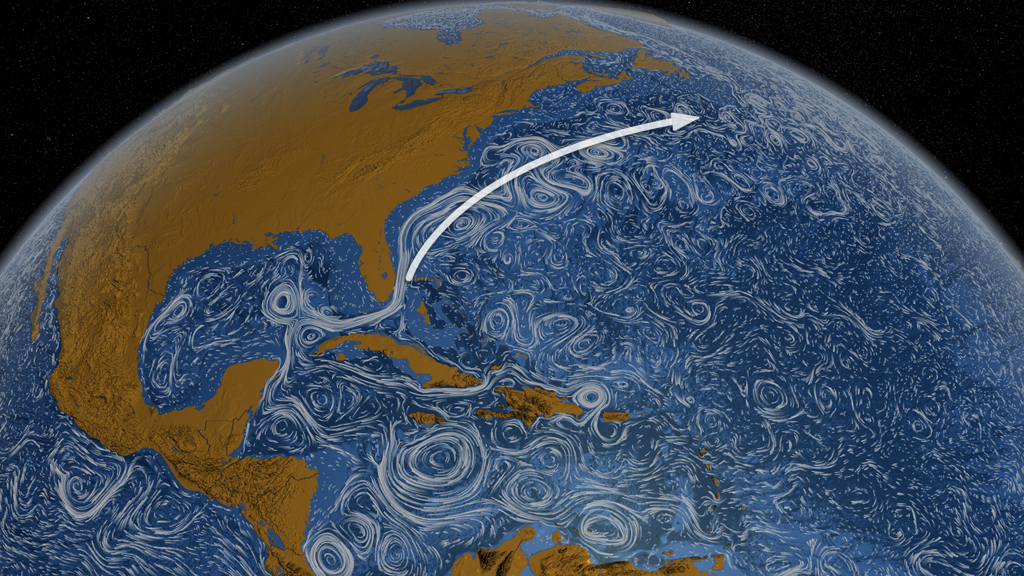
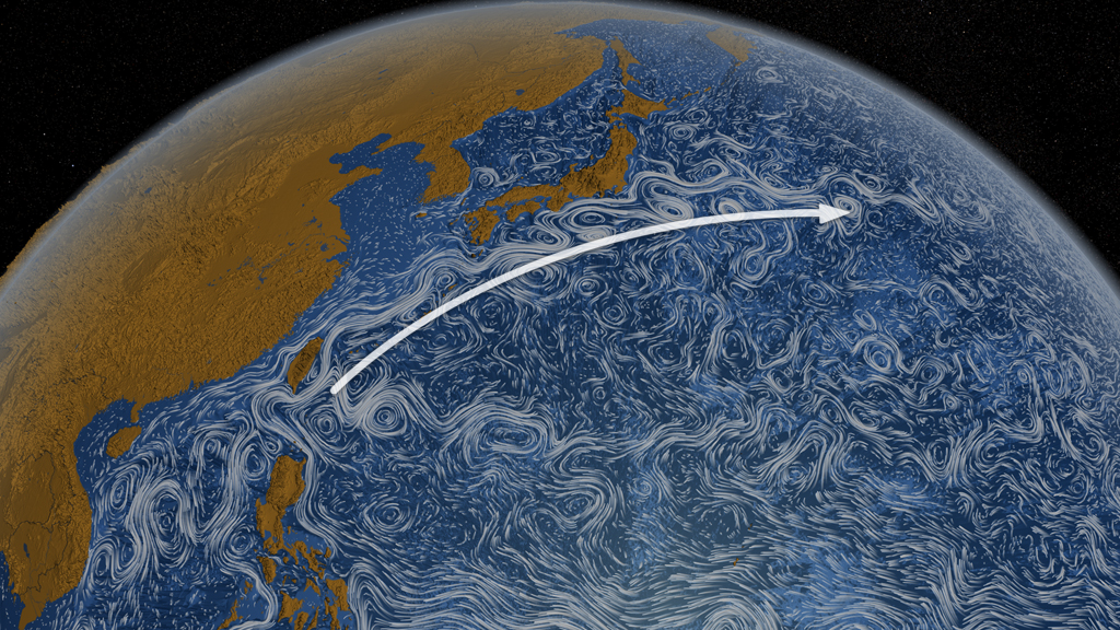
Since geostrophy is the dominant balance underneath the mixed layer, it is convenient to define: \[ u = -\Psi_y, \quad v = \Psi_x, \quad \text{where } \Psi = \frac{p}{\rho_0 f_0}, \quad \text{the streamfunction} \] Form the vorticity equation by \((II)_y - (I)_x\) (as before, but now complete, with all the terms): $$ \zeta_t + \vec{u} \cdot \nabla \zeta + \beta v = (f_0 + \beta y + \zeta) w_z + k_H \nabla^2 \zeta $$ With $\zeta$ being the relative vorticity, $$ \zeta = v_x - u_y = \nabla^2 \Psi $$ Exploiting that $f_0 \ll \beta y + \zeta$ (why?) and integrating from top to bottom: $$ \zeta_t + \vec{u} \cdot \nabla \zeta + \beta v = \frac{f_0}{D}(w_E - w_B) + k_H \nabla^2 \zeta $$ Three Extra Terms!! $$ \zeta_t + \vec{u} \cdot \nabla \zeta + \beta v = \frac{f_0}{D}(w_E - w_B) + k_H \nabla^2 \zeta $$ There is now also an Ekman layer at the bottom of the ocean, but here the friction depends on the flow, i.e., it is part of the solution. At the surface, the stress caused by flow is independent of the flow, since $U_{\text{wind}} \gg U_{\text{ocean}}$. Let's assume: $$ \tau^x_{\text{Bottom}} = \alpha u, \quad \tau^y_{\text{Bottom}} = \alpha v $$ Analogous to the surface Ekman pumping, we then have a bottom Ekman pumping: $$ w_B = -\frac{\alpha}{\rho_0 f}(v_x - u_y) $$ So we replace $\frac{f_0}{D} w_B$ with: $$ r \nabla^2 \psi, \text{ where } r \text{ is a decay rate (think } \zeta_t = -r \nabla^2 \psi \text{)} $$ The Kuroshio Current and the Gulf Stream are two of the most well-known western boundary warm currents in the global ocean and play a critical role in influencing global climate change. It is precisely due to the influence of the North Atlantic Current — an extension of the Gulf Stream—that northwestern Europe experiences a consistently mild and humid climate. The Gulf Stream transports approximately 113 million cubic meters of water per second, while the Kuroshio Current can travel 25 to 75 miles per day, with a volume comparable to that of 6,000 major rivers.
NASA created a video titled Perpetual Ocean, which vividly shows the movement of ocean currents in great detail, it is very stunning.

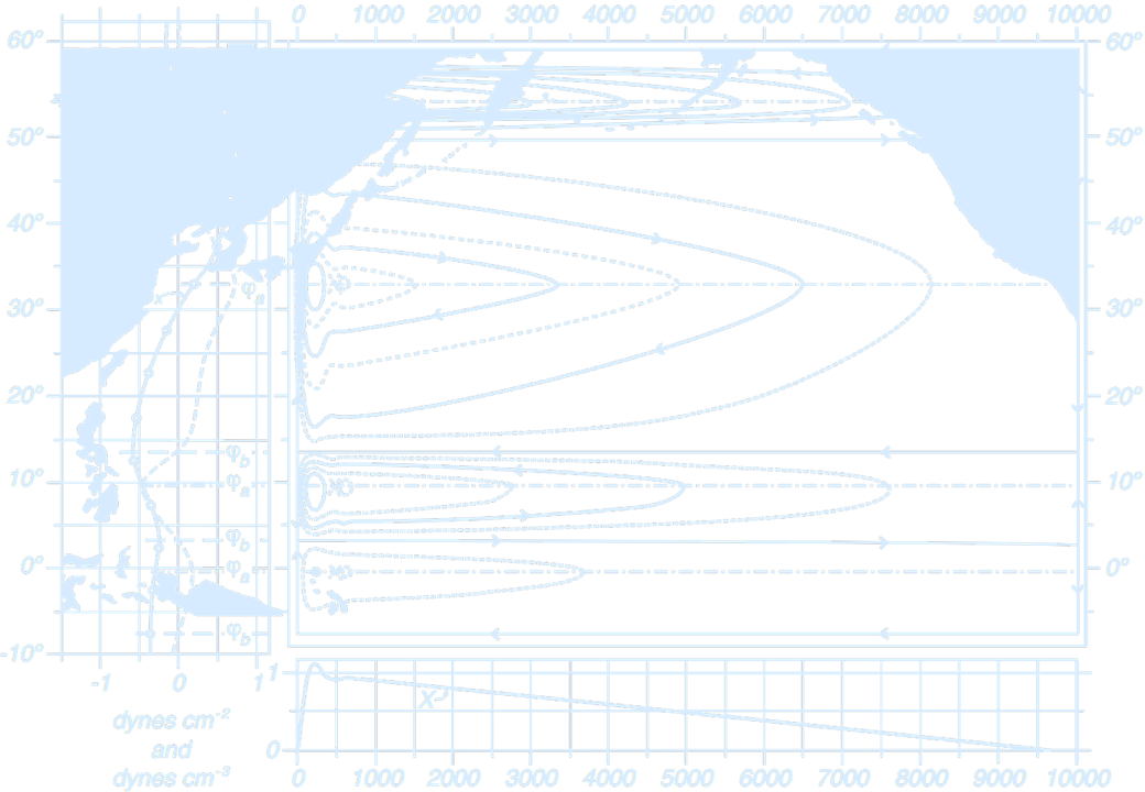
Western Intensification

The westerlies of middle latitudes and the trade winds of the tropics drive the most prominent features of ocean surface motion, large-scale roughly circular current systems elongated in the east-west direction known as gyres.

• Water moving eastward (in the westerly winds band) is deflected more than water moving westward (in the trade winds zone)
• Westerly zone → water is transported towards the gyre center over the entire ocean width
• Trade wind zone → little deflection; flow pushes water to west side of the ocean
• Gyre center is offset to the west
• Pressure gradient is larger on the west side (steeper slope) → stronger geostrophic currents

Note that the western boundary currents of all subtropical gyres are western intensified, even in the Southern Hemisphere.

Stream Field

Stream field in any significant small area can be considered as a set of four basic elementary stream areas: translation, rotation, divergence, and deformation [12].

• Streamlines: Line represents the linear curve which is tangential with the local vector current speed.
• Translator field: Because the speed of flow is the vector size, translator field represents movement through the displacement vector field for translation. The fluid moves around the same speed and direction and intensity. Streamlines lie in the direction of flow are the parallel lines. That stream field does not change the volume or shape of the fluid.
• Rotation field: Streamlines are concentric circles. The fluid rotates around a common centre of stream field. The speed of flow increases linearly with increasing distance of streamlines from the centre of rotation. During the rotation, individual air particles do not change its shape or volume.
• Divergence and convergence field: Streamlines are straight and pass through the centre of the field as a joint stream point. When fluid flows towards the centre, flow is convergent, and the point is called convergent point. If the flow is done from the center to the field, it is called the point of divergence. The convergence of a fluid particle does not alter its shape, while both the rate of flow and volume of particle are going to reduce the convergence point. In the divergence, flow is from the centre towards the outer area, the flow increases its velocity and volume, but particles in this case do not change their shape.
• Deformation field: Streamlines are concentric equilateral hyperbolas and their velocity increases linearly in any direction from the center to the field. Linear speed of the centre field linearly increases. Movement does not change the volume of the fluid particle, but it changes its shape. When approaching the common center of the hyperbola (center of the field), the dimensions of the particles decrease in the direction of flow, and when moving away from the center, the dimensions of the particles increase in the direction of flow.

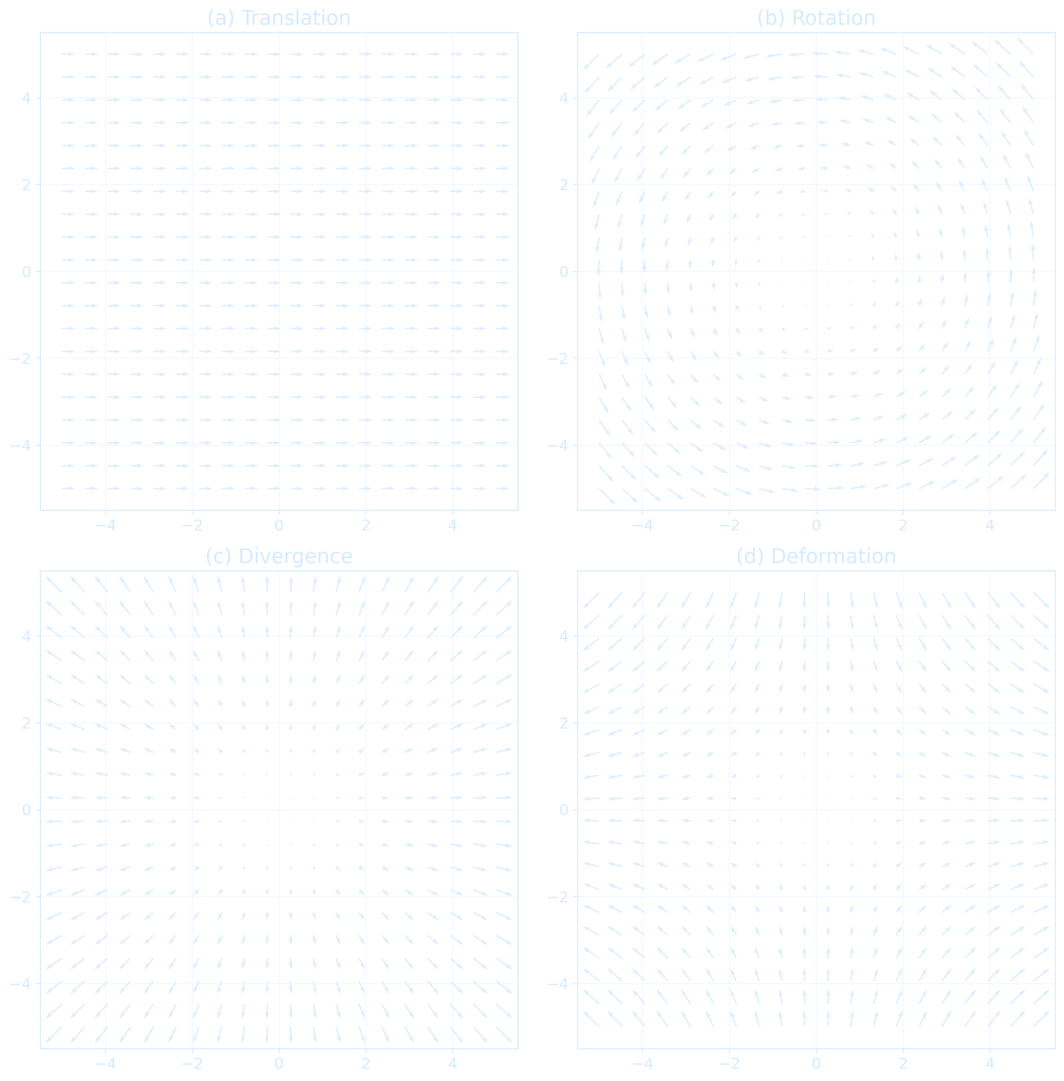
Vorticity Equation

Since the horizontal velocity is divergence-free (because of the flat-bottom and rigid-lid) we may represent it as a streamfunction \(\psi\). Our full vorticity equation rewritten with \(\psi\) is: \[ \overbrace{ \underbrace{\frac{\partial}{\partial t} (\nabla^2 \psi)}_{\text{Local change of relative vorticity } \zeta = \frac{\partial v}{\partial x} - \frac{\partial u}{\partial y}} + \underbrace{J(\psi, \nabla^2 \psi)}_{\text{Jacobian, Nonlinear advection of vorticity}} }^{\text{Material derivative } \frac{D\zeta}{Dt}} + \underbrace{\beta \psi_x}_{\text{Meridional advection of planetary vorticity}} = \underbrace{\frac{f_0}{D} w_E}_{\text{Column Stretching/compression by Ekman pumping}} - \underbrace{r \nabla^2 \psi}_{\text{Linear bottom friction}} + \underbrace{k_H \nabla^4 \psi}_{\text{Horizontal friction}} \] with \[J(A, B) = A_x B_y - A_y B_x\]

The Depth Integrated Wind-driven Circulation

We now have 3 extra physical processes to break the Sverdrup balance, and close the circulation: bottom friction, sidewall friction, and advection. Advection may be important locally, but obviously somewhere friction has to remove the vorticity that wind has put into the system. So let’s look for a solution with friction first:
Stommel 1948: $$ \beta \Psi_x = \frac{f_0}{D} w_E - r \nabla^2 \Psi $$ Munk 1950: $$ \beta \Psi_x = \frac{f_0}{D} w_E + k_H \nabla^4 \Psi $$ Practice with Stommel: $$ \Psi_{xx} \gg \Psi_{yy} \quad \Longrightarrow \quad \beta \Psi_x = \frac{f_0}{D} w_E - r \Psi_{xx} $$ We still cannot solve that, but can use perturbation methods, developed in the late fourties ;-)

Stommel's Solution

$$ \Psi_{xx} \gg \Psi_{yy} \Longrightarrow \beta \Psi_x = \frac{f_0}{D} w_E - r \Psi_{xx} $$ Let $\Psi = \Psi^S + \Psi^W$, with $\Psi^S = \frac{f_0}{\beta D} \int_x^{x_E} w_E \, dx$ and $\Psi = 0$ at $x = 0$, $\Psi = \Psi^S$ for large $x$. $$ \Rightarrow \quad r \Psi^W_{xx} + \beta \Psi^W_x = 0 $$ $$ \Rightarrow \quad \Psi^W = -\Psi^S e^{-x/\delta_S}, \quad \text{and} \quad \Psi = \Psi^S (1 - e^{-x/\delta_S}) $$ with \(\boxed{\delta_S = \beta / r}\), the Stommel boundary layer width $$ \Rightarrow \quad v = \Psi_x = v_s + \frac{1}{\delta_S} e^{-x/\delta_S} $$ Stommel’s assumption:

• Include only linear bottom drag: keep $-r \nabla^2 \psi$
• Ignore $\nabla^4 \psi$ and nonlinear terms

$$ \overbrace{ \cancel{ \underbrace{\frac{\partial}{\partial t} (\nabla^2 \psi)}_{\text{Local change of relative vorticity } \zeta}} + \cancel{ \underbrace{J(\psi, \nabla^2 \psi)}_{\text{Nonlinear advection of vorticity}}} }^{\text{Material derivative } \frac{D\zeta}{Dt}} + \underbrace{\beta \frac{\partial \psi}{\partial x}}_{\text{Meridional advection of planetary vorticity}} = \underbrace{\frac{f_0}{D} w_E}_{\text{Ekman pumping (stretching/compression)}} - \underbrace{r \nabla^2 \psi}_{\text{Linear bottom friction}} + \cancel{ \underbrace{k_H \nabla^4 \psi}_{\text{Horizontal friction}}} $$ Resulting vorticity equation: $$ \beta \frac{\partial \psi}{\partial x} = \frac{f_0}{D} w_E - r \nabla^2 \psi $$ In the western boundary layer , we assume variation in $x$ is much stronger than in $y$: $$ \psi_{xx} \gg \psi_{yy} \Rightarrow \beta \psi_x = \frac{f_0}{D} w_E - r \psi_{xx} $$ Using full derivatives notation: $$ \frac{\partial^2 \psi}{\partial x^2} \gg \frac{\partial^2 \psi}{\partial y^2} \quad \Rightarrow \quad \boxed{ \beta \frac{\partial \psi}{\partial x} = \frac{f_0}{D} w_E - r \frac{\partial^2 \psi}{\partial x^2} } $$

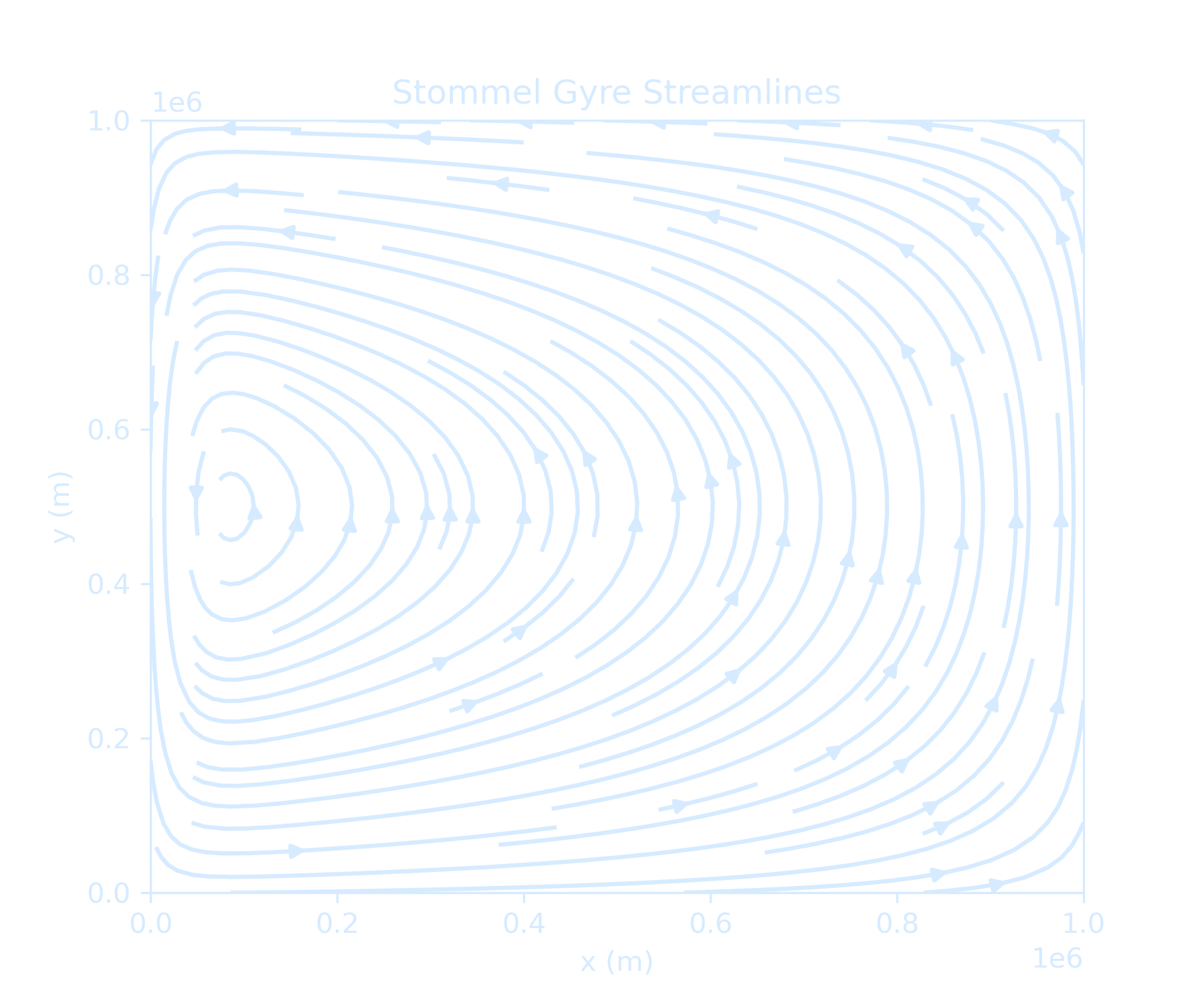
Munk's Solution

$$ \Psi_{xx} \gg \Psi_{yy} \Longrightarrow \beta \Psi_x = \frac{f_0}{D} w_E + k_H \Psi_{xxxx} $$ Let $\Psi = \Psi^S + \Psi^W$, with $$ \Psi^S = \frac{f_0}{\beta D} \int_x^{x_E} w_E \, dx $$ and $\Psi = 0$ at $x = 0$, $\Psi = \Psi^S$ for large $x$.
We need more boundary conditions though!
No slip: $\Psi_x = v = 0$ at $x = 0$
Free slip: $\Psi_{xx} = v_x = 0$ at $x = 0$
The most general solution to Munk’s vorticity equation: $$ \Psi = \Psi^S \left(1 - e^{\frac{-x}{2 \delta_M}} \cos\left(\sqrt{3}/2 \delta_M x\right)\right) + C(y) \, e^{\frac{-x}{2 \delta_M}} \sin\left(\sqrt{3}/2 \delta_M x\right) $$ with \(\boxed{\delta_M = \left(\frac{k_H}{\beta}\right)^{1/3}}\), the Munk boundary layer width, C(y) has to be determined as a function of the boundary conditions: $$ \Psi = \Psi^S \left(1 - e^{\frac{-x}{2 \delta_M}} \cos\left(\sqrt{3}/2 \delta_M x\right)\right) \pm \frac{1}{\sqrt{3}} \sin\left(\sqrt{3}/2 \delta_M x\right) $$ Munk’s extension:

• Adds horizontal friction using biharmonic term $+k_H \nabla^4 \psi$
• Important for resolving realistic boundary layers

$$ \overbrace{ \cancel{ \underbrace{\frac{\partial}{\partial t} (\nabla^2 \psi)}_{\text{Local change of relative vorticity } \zeta}} + \cancel{ \underbrace{J(\psi, \nabla^2 \psi)}_{\text{Nonlinear advection of vorticity}}} }^{\text{Material derivative } \frac{D\zeta}{Dt}} + \underbrace{\beta \frac{\partial \psi}{\partial x}}_{\text{Meridional advection of planetary vorticity}} = \underbrace{\frac{f_0}{D} w_E}_{\text{Column Stretching/compression by Ekman pumping}} - \underbrace{\cancel{r \nabla^2 \psi}}_{\text{Linear bottom friction}} + \underbrace{k_H \nabla^4 \psi}_{\text{Horizontal friction}} $$ Applying the western boundary layer assumption: $$ \nabla^4 \psi \approx \frac{\partial^4 \psi}{\partial x^4} \quad \Rightarrow \quad \boxed{ \beta \frac{\partial \psi}{\partial x} = \frac{f_0}{D} w_E + k_H \frac{\partial^4 \psi}{\partial x^4} } $$

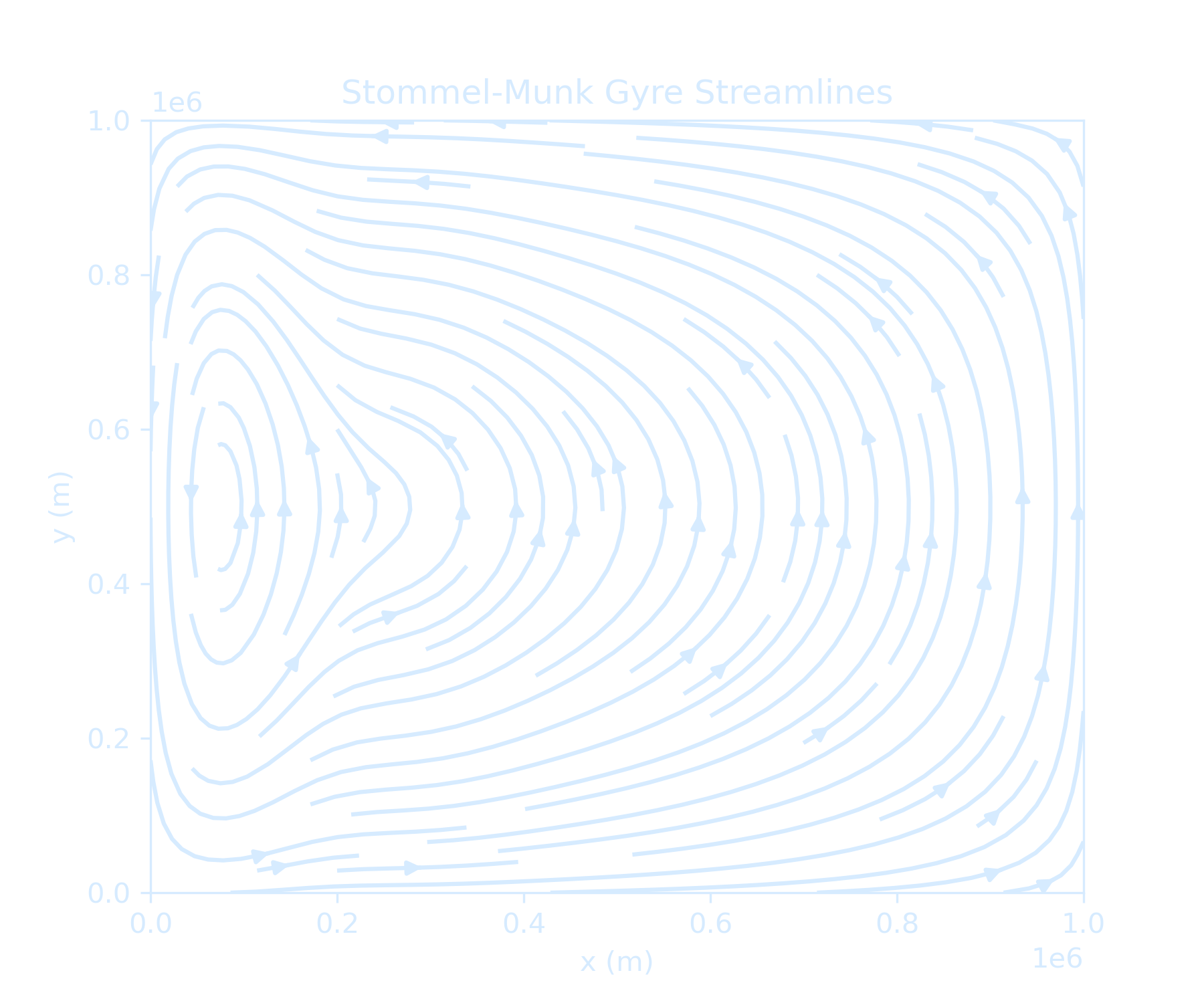
Eastern Boundary Currents

Wind-induced Ekman transport causes surface waters to converge and downwell in the western part of ocean basins, creating a zonal pressure gradient that drives geostrophic currents toward the western boundary. To return to higher latitudes, the flow must gain positive planetary vorticity. The sidewall friction of the western boundary can provide this, whereas the eastern boundary can only provide negative vorticity. Therefore, intensified currents must occur on the western boundary.
Eastern boundary currents of major ocean basins are mainly upwelling currents caused by persistent trade winds blowing along the coast. Below are some important eastern boundary currents:

Name	Region
California Current	Pacific
Peru Current	Pacific
Western Australian Current	Indian
Benguela Current	Atlantic
Canary Current	Atlantic

Next: Project 3 – Western Boundary Currents