Project 2 – The Sverdrup Relation

Use the ACC setup of Veros to test the Sverdrup theory.

Show the model’s stream function and compare it to the theory’s.
Make sure the model is spun up, and be careful with the units.

Where does the model deviate from the theory and why?

Ocean Modelling with Veros

Running Veros on ERDA

cd ~/erda_mount

/home/jovyan/erda_mount

!git clone https://github.com/team-ocean/veros.git -b v1.5.2

cd veros

/home/jovyan/erda_mount/veros

conda env create -f conda-environment.yml

Inside the ERDA Jupyter notebook, you cannot do conda activate veros normally, because Jupyter runs inside its own kernel. If you want to properly activate the Veros conda environment and run Veros, you must open a Terminal on ERDA. In the Terminal, type:

conda activate veros

To tell Veros what to do, you need to write a so-called setup, create your setups

mkdir ~/vs-setups
cd ~/vs-setups
veros copy-setup global_4deg
cd global_4deg

Right now, your default global_4deg.py has settings.runlen = 0, which means "run for 0 seconds". Edit the setup file to actually run for longer

settings.runlen = 86400 * 365 * 10  # 10 model years, = 10 years × 365 days × 86400 seconds/day

Now run the simulation

veros run global_4deg.py

veros run global_4deg.py
Importing core modules
 Using computational backend numpy on cpu
 Runtime settings are now locked

Running model setup
 removing an annual mean heat flux imbalance of 7.860702e-02 W/m^2
Initializing streamfunction method
Computing ILU preconditioner...
 Solving for boundary contribution by island 0
 Solving for boundary contribution by island 1
 Solving for boundary contribution by island 2
 Solving for boundary contribution by island 3
 Solving for boundary contribution by island 4
 Solving for boundary contribution by island 5
 Running diagnostic "averages" every 1.0 days
 Writing output for diagnostic "averages" every 1.0 years
 Running diagnostic "energy" every 1.0 days
 Writing output for diagnostic "energy" every 1.0 years
 Running diagnostic "overturning" every 1.0 days
 Writing output for diagnostic "overturning" every 1.0 years
 Writing output for diagnostic "snapshot" every 1.0 years
Diffusion grid factor delta_iso1 = 0.013376791936035174

Starting integration for 10.0 years
 Writing snapshot at 1.00 years                                                  
 Writing snapshot at 2.00 years                                                  
 Writing snapshot at 3.00 years                                                  
 Writing snapshot at 4.00 years                                                  
 Writing snapshot at 5.00 years                                                  
 Writing snapshot at 6.00 years                                                  
 Writing snapshot at 7.00 years                                                 
 Writing snapshot at 8.00 years                                                 
 Writing snapshot at 9.00 years                                                 
 Writing snapshot at 10.00 years                                                  
 Current iteration: 3600  (10.00/10.00y | 100.0% | 2.38m/(model year) | 0.0s left)
Integration done

Writing restart file global_4deg_3600.restart.h5

It should be noted that Veros cannot overwrite an existing file by default, so if you want to re-run the same script, do something like :

rm -rf global_4deg
veros copy-setup global_4deg
cd global_4deg

rm global_4deg.*.nc global_4deg_*.restart.h5

To generate new output filenames (e.g., global_4deg_modified.averages.nc, etc.), change the runtime settings.identifier string in your setup file such as modify_global_4deg.py to something like:

settings.identifier = "global_4deg_modified"

After a successful run, Veros writes NetCDF files in the current folder ~/vs-setups/global_4deg/. You will find files like: global_4deg.snapshot.nc, global_4deg.averages.nc, global_4deg.energy.nc, global_4deg.overturning.nc, global_4deg_0000.restart.h5. In your notebook, you can load Veros output

import os
os.chdir("/home/jovyan/vs-setups/global_4deg")  # Go to correct directory

import xarray as xr
import matplotlib.pyplot as plt
import cmocean

ds = xr.open_dataset("global_4deg.snapshot.nc", engine="h5netcdf")

# Extract surface temperature
temp_surface = ds.temp.isel(Time=-1, zt=-1)

# Start plot
fig, ax = plt.subplots(figsize=(8, 5), facecolor="none", dpi=300)  # transparent background

# Plot with cmocean thermal colormap
p = temp_surface.plot.pcolormesh(
    ax=ax,
    cmap=cmocean.cm.thermal,
    add_colorbar=True,
    cbar_kwargs={"label": "Temperature (°C)", "orientation": "vertical"},
)

# Set color
text_color = "#d6ebff"
ax.set_title("Surface Temperature", color=text_color)
ax.set_xlabel("Longitude", color=text_color)
ax.set_ylabel("Latitude", color=text_color)

# Set tick params
ax.tick_params(axis="both", colors=text_color)

# Set axis spines color (frame lines)
for spine in ax.spines.values():
    spine.set_edgecolor(text_color)

# Set colorbar text and frame color
cbar = p.colorbar
cbar.ax.yaxis.label.set_color(text_color)
cbar.ax.tick_params(colors=text_color)
# Set colorbar outline (the frame)
cbar.outline.set_edgecolor(text_color)

# Transparent background
ax.set_facecolor("none")
fig.patch.set_alpha(0.0)  # fully transparent

fig.savefig("surface_temperature.png", dpi=300, bbox_inches="tight", transparent=True)
# Show plot
plt.show()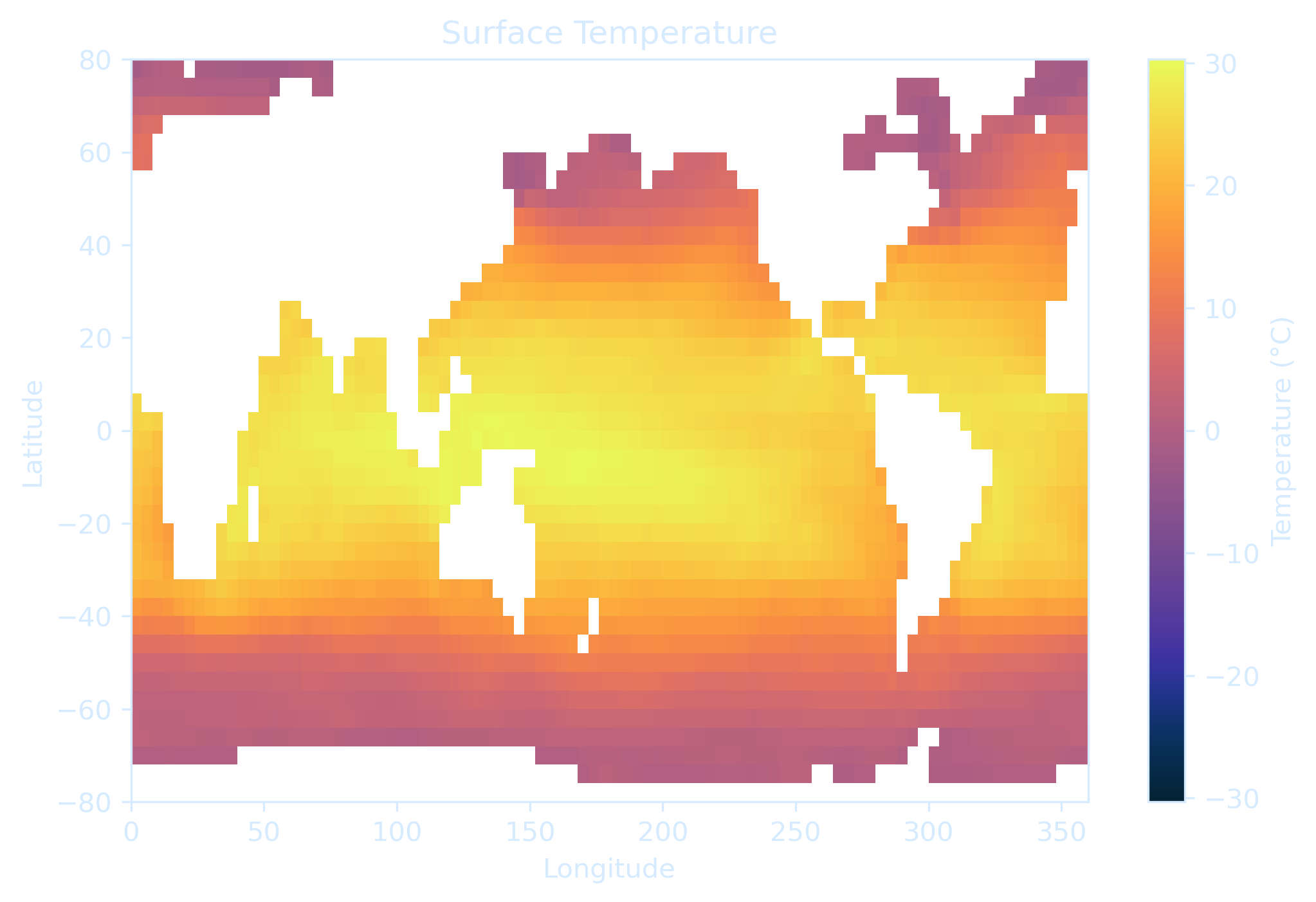

Now let's start with your own script

cd ~/vs-setups/
mkdir acc_basic
cd acc_basic

Save the script acc_basic.py inside this folder, if you are using Jupyter Notebook, in a notebook cell, write:

%%writefile acc_basic/acc_basic.py

from veros import VerosSetup, veros_routine
from veros.variables import allocate, Variable
from veros.distributed import global_min, global_max
from veros.core.operators import numpy as npx, update, at
# (the rest of the script)

Then to run, your output NetCDF files will also be inside ~/vs-setups/acc_basic/:

conda activate veros
veros run acc_basic.py --force-overwrite

Importing core modules
 Using computational backend numpy on cpu
 Runtime settings are now locked

Running model setup
Initializing streamfunction method
Computing ILU preconditioner...
 Solving for boundary contribution by island 0
 Solving for boundary contribution by island 1
 Running diagnostic "averages" every 5.0 days
 Writing output for diagnostic "averages" every 1.0 years

Starting integration for 50.7 years
 Current iteration: 36500 (50.69/50.69y | 100.0% | 29.55s/(model year) | 0.0s left)
Integration done

Writing restart file acc_sverdrup_36500.restart.h5

There are many predefined setups in Veros, so you will not have to write one from scratch, you can also do

veros copy-setup acc

If you want a fresh copy, remove the existing acc/ folder and copy again:

rm -rf acc
veros copy-setup acc

Then just go inside the acc/ folder and run it, make sure the file path is correct

veros run acc/acc.py

Load output and inspect $\Psi$

Plot the 1D curve of the maximum value of $\Psi$ over time and check whether the model is fully spun up, ie. whether it has reached the steady state.

ds['psi'].max(dim=("xu", "yu")).plot()

If you are satisfied with the plot, go ahead and re-define 'ds' as the last model year of the original output set.

ds = ds.isel(Time=-1)

Compute wind stress curl

Define $\rho_0$, $\Omega$ and the Earth's radius, $a$

#rho_0 = 
#omega = 
#earth_radius = 
#beta = 2 * omega * np.cos(np.radians(ds['yu'].values)) / earth_radius

Now you need to export and define some variables from the output set. Namely, the output barotropic stream function to compare with the computed $\Psi_{Sv}$, and the grid coordinates $x$ and $y$. The values() method is one of the Python Dictionary Methods, it returns a list of all the values in the dictionary. The view object contains the values of the dictionary, as a list. Define variables psi, yt and xt from ds.

#course = {
  #"university": "UCPH",
  #"name": "Computational Atmosphere and Ocean Dynamics",
  #"code": "NFYK22003U",
  #"year": 2025
#}

#x = course.values()

#print(x)

Correct the definitions below to express $dx$ and $dy$ in meters

dx = (xt[1] - xt[0]) * np.cos(np.radians(yt))
dy = (yt[1] - yt[0])

The following two functions can integrate and compute the gradient of an array. The function integrate takes 3 arguments: the array you wish to integrate over, the direction (either $x$ or $y$), and a boolean variable which, when set to True, will flip the limits of the integral. For example, if we have: \[ \int^{x_1}_{x_0} f(x,y) dx, \] setting the variable reverse=True will result in the function output $\int_{x_1}^{x_0} f(x,y) dx$. The function gradient takes 2 arguments: the array you wish to differentiate over, and the direction (either $x$ or $y$). Let the imput function be $g(x,y)$ and the direction $x$, the function output is then: \[ \frac{\partial}{\partial x} g(x,y) \]

def integrate(q, direction, reverse=False):
    if direction == 'x':
        dxi = dx[:, np.newaxis]
        axis = 1
        
        if reverse:
            q = q[:, ::-1]
            
    elif direction == 'y':
        dxi = dy
        axis = 0
        
        if reverse:
            q = q[::-1]
            
    else:
        raise ValueError('direction must be "x" or "y"')
        
    out = np.nancumsum(q * dxi, axis=axis)
    out[np.isnan(q)] = np.nan
    
    if reverse:
        if direction == 'x':
            out = -out[:, ::-1]
        else:
            out = -out[::-1, :]
        
    return out


def gradient(q, direction):
    """Compute the gradient of a 2D variable on a C-grid"""
    if direction == 'x':
        arr_pad = np.pad(q, ([0], [1]), 'wrap')
        return (arr_pad[:, 2:] - arr_pad[:, 1:-1]) / dx[:, np.newaxis]

    elif direction == 'y':
        arr_pad = np.pad(q, ([1], [0]), 'constant', constant_values=np.nan)
        return (arr_pad[2:, :] - arr_pad[1:-1, :]) / dy

    raise ValueError('direction must be "x" or "y"')

Use a suitable function to compute $\nabla \times \tau$. Hint: The definition of a curl in 2D is $\nabla \times f(x,y) = \frac{\partial}{\partial x} f_y(x,y) - \frac{\partial}{\partial y} f_x(x,y)$

Check your solution by ploting $\nabla \times \tau$. Does the calculated $\nabla \times \tau$ make sense? Why?

Compute $\Psi_\text{Sv}$ and compare

Well done so far, you are almost there! The task is now to compare the output barotropic streamfunction ds['psi'] to the $\Psi_{Sv}$ calculated from: \[ \Psi_{Sv} = \int_{East}^{West}V_{Sv}dx \] Note that the integral goes from East to West, as the boundary wall is placed on the eastern end of the basin.
Use the definition of $V_{Sv}$ to compute it from the defined constants and the calculated curl of $\tau$. Then, compute the barotropic stream function $\Psi_{Sv}$ and compare it to the $\Psi$ from the model output by examining their successive plots.

It should be noted that mathematically, a reverse integration over a variable (integrating from right to left) is not the same as just flipping the input and calling np.cumsum() — you need to negate the result too. Because if you are integrating a function $f(x)$ on a discrete 1D grid with uniform spacing $\Delta x > 0$, your discrete integral becomes a sum: \[ \int_{x_0}^{x_n} f(x)\,dx \approx \sum_{i=0}^{n-1} f_i \, \Delta x \] This is equivalent to np.cumsum(f * dx) in NumPy. Let

$f = [f_0, f_1, f_2, f_3]$
$\Delta x > 0$

Then the cumulative integral is: $ \text{cumint}[0] = f_0 \Delta x $
$\text{cumint}[1] = (f_0 + f_1) \Delta x $
$\text{cumint}[2] = (f_0 + f_1 + f_2) \Delta x $
$\text{cumint}[3] = (f_0 + f_1 + f_2 + f_3) \Delta x $
This is what np.cumsum(f * dx) does. Now suppose you want to integrate right to left (from $x_n$ to $x_0$): \[ \int_{x_n}^{x_0} f(x)\,dx = - \int_{x_0}^{x_n} f(x)\,dx \] If you do


np.cumsum(f[::-1] * dx)[::-1]

you're computing the values of integration in reverse order, but the sign is still assuming $x_0 \to x_n$, not $x_n \to x_0$. You’re essentially computing:
$ \text{bad_reverse}[0] = (f_3) \Delta x $
$\text{bad_reverse}[1] = (f_3 + f_2) \Delta x $
$\text{bad_reverse}[2] = (f_3 + f_2 + f_1) \Delta x $
$\text{bad_reverse}[3] = (f_3 + f_2 + f_1 + f_0) \Delta x$
Then reversing the array order doesn't fix the fact that this is still a positive integral, just with terms accumulated in reverse. Because you're still summing the same values — just in reverse. But the limits of integration are reversed, so you must negate the sum to account for this. To compute the correct integral from $x_n$ to $x_0$ \[ \int_{x_n}^{x_0} f(x)\,dx = -\sum_{i=0}^{n-1} f_i \Delta x \] So your NumPy expression must include a negation:


- np.cumsum(f[::-1] * dx)[::-1]

Conclusions

How does the diagnostic streamfunction differ from the one calculated from the Sverdrup balance?
How do these two solutions compare in the open ocean vs. at the boundaries?
How well does this idealized model reflect real winds and ocean currents?