Project 4 – Shadow Zone
Does the thermocline theory explain the oxygen minimum zone?
- Identify the oxygen minimum zones in the data set that you used for project 1.
- In the North Pacific part of the data, define three density classes with which you can
construct a three layer model of the subtropical gyre, and create a sinusoidal Ekman
pumping field ( i.e., something based on
taux = A cos (Pi * y/L)). - Use the theory derived in class to determine the structure of the shadow zone, and compare it with the shape of the oxygen minimum zone.
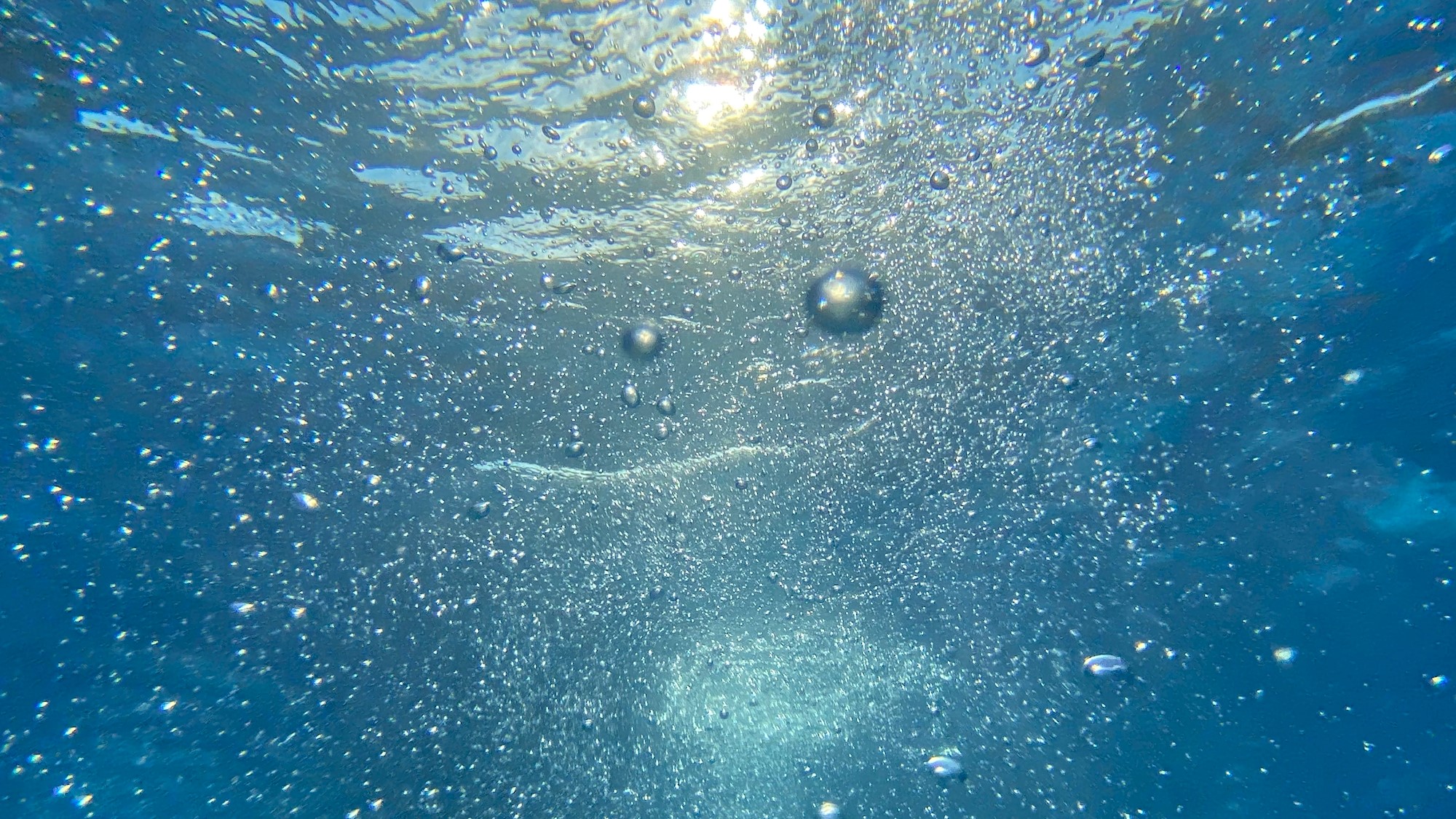
(Ocean mixing and the interaction of currents govern oxygen availability and determine how and when it’s used. Credit: J K/Unsplash)
The thermocline theory can be tested by theocean.nc on Absalon using Community Earth System Model (CESM) 100 year average output from a fully coupled simulation with ocean, atmosphere, land, sea ice and biogeochemistry components. The model grid resolution varies with latitude, with a total of 100×118 grid points and 60 depth levels.
A theoretical box is set up within the output domain, which is meant to capture the extent of the northern subtropical gyre in the Pacific Ocean. The extent of the box along the meridional direction is determined by finding two points at which the Ekman transport is zero, defined as:
$$
w_E = \frac{1}{\rho_0} \nabla \times \left( \frac{\tau}{f} \right) = \frac{1}{\rho_0} \left( \frac{\partial}{\partial x} \frac{\tau_y}{f} - \frac{\partial}{\partial y} \frac{\tau_x}{f} \right)
$$
where $\rho_0$ is the density of salt water, $\tau$ is the horizontal wind stress vector and $f$ is the Coriolis parameter. The magnitude of the zonal winds is an order of magnitude larger than the meridional winds, therefore the Ekman transport simplifies to:
$$
w_E = -\frac{1}{\rho_0} \frac{\partial}{\partial y} \left( \frac{\tau_x}{f} \right)
$$
The wind stress is further simplified by computing the zonal average and assuming that $w_e$ is constant in the zonal direction. The idealized ocean within the box has three density layers, the top light layer, the subducted layer and the stagnant abyss. The thermocline theory states that:
$$
D^2 = H^2 \frac{\gamma_1}{\gamma_2} \left(1 - \frac{f}{f_2} \right)^2
$$
where $H$ is the height of the subducted layer at the point of subduction, $f_2$ is the Coriolis parameter at the point of subduction, $\gamma_1$ and $\gamma_2$ are the reduced gravities of the top two layers, and
$$
D^2 = -\frac{2f^2}{\beta \gamma_2} \int_x^{x_E} w_E dx
$$
with the Rossby parameter $\beta$ and the reduced gravity of the subducted layer $\gamma_2$. In our idealized case $w_E$ is independent of $x$, therefore $D^2$ reduces to:
$$
D^2 = -\frac{2f^2}{\beta \gamma_2} w_E (x_E - x)
$$
and combining with equations \(\boxed{w_E = -\frac{1}{\rho_0} \frac{\partial}{\partial y} \left( \frac{\tau_x}{f} \right)}\) and \(\boxed{D^2 = H^2 \frac{\gamma_1}{\gamma_2} \left(1 - \frac{f}{f_2} \right)^2}\), we can solve for $x$:
$$
x_E - x = H^2 \left(1 - \frac{f}{f_2} \right)^2 \frac{\beta \gamma_1 \rho_0}{2 f^2} \frac{1}{\frac{\partial (\tau_x / f)}{\partial y}}
$$
This equation can be used to trace the zonal distance from the Eastern boundary $x_E$ of the subducted layer in the interior of the ocean, and thereby determine the shape of the shadow zone.
Next: Lecture 8 – Waves