Maths Speedrun
Differentiation
In physics, differentiation are used to describe phenomena, and the reason might be: the core of physics research is change, and differentiation is the mathematical tool used to describe change.In the following we assume that $C$ and $a$ are constants.
- $\frac{d}{dx}(C) = 0$;
- $\frac{d}{dx} x^n = nx^{n-1}$;
- $\frac{d}{dx} \sin x = \cos x$;
- $\frac{d}{dx} \cos x = -\sin x$;
- $\frac{d}{dx} \log_a x = \frac{\log_a e}{x}$; where $a > 0, a \neq 1$;
- $\frac{d}{dx} \ln x = \frac{1}{x}$;
- $\frac{d}{dx} a^x = a^x \ln a$;
- $\frac{d}{dx} e^x = e^x$.
- $\frac{d}{dx} \{ f(x) + g(x) \} = \frac{d}{dx} f(x) + \frac{d}{dx} g(x) = f'(x) + g'(x)$ (Addition Rule)
- $\frac{d}{dx} \{ f(x) - g(x) \} = \frac{d}{dx} f(x) - \frac{d}{dx} g(x) = f'(x) - g'(x)$ (Subtraction Rule)
- $\frac{d}{dx} \{ C f(x) \} = C \frac{d}{dx} f(x) = C f'(x)$ where $C$ is a constant
- $\frac{d}{dx} \{ f(x) g(x) \} = f(x) \frac{d}{dx} g(x) + g(x) \frac{d}{dx} f(x) = f(x) g'(x) + g(x) f'(x)$ (Product Rule)
- $ \frac{d}{dx} \left\{ \frac{f(x)}{g(x)} \right\} = \frac{g(x) \frac{d}{dx} f(x) - f(x) \frac{d}{dx} g(x)}{[g(x)]^2} = \frac{g(x) f'(x) - f(x) g'(x)}{[g(x)]^2} $ if $g(x) \neq 0$ everywhere.
[Ex] Product Rule $$ \frac{d}{dx} \{ x \sin x \} = x \frac{d}{dx} \sin x + \sin x \frac{d}{dx} x $$ $$ = x \cos x + \sin x $$ [Ex] Quotient Rule $$ \frac{d}{dx} \tan x = \frac{d}{dx} \left\{ \frac{\sin x}{\cos x} \right\} $$ $$ = \frac{\cos x \frac{d}{dx} \sin x - \sin x \frac{d}{dx} \cos x}{(\cos x)^2} $$ $$ = \frac{1}{(\cos x)^2} $$ [Q]$ \frac{d}{dx} \arcsin x = \boxed{?} $
[Sol] (Let $y = \arcsin x$) $$ \frac{d}{dx} \arcsin x = \frac{dy}{d \sin y} = \frac{1}{\frac{d \sin y}{dy}} $$ $$ = \frac{1}{\cos y} = \frac{1}{\sqrt{1 - \sin^2 y}} = \frac{1}{\sqrt{1 - x^2}} $$ [Q] Find $ \frac{dy}{dx} = \boxed{?} \quad \text{where } y = \sin(t^2), \quad x = 1 + \sqrt{t}. $
[Sol]$$ \frac{dy}{dx} = \frac{(\sin(t^2))'}{(1 + \sqrt{t})'} $$ $$ = \frac{2t \cos(t^2)}{\frac{1}{2\sqrt{t}}} $$ $$ = 4t^{\frac{3}{2}} \cos(t^2) $$ Derivatives of Commonly Used Functions: In the following we assume that u is a differentiable function of x. With the rules for differentiation and the derivatives of elementary functions mentioned before, we have the following derivatives of functions.
- $ \frac{d}{dx} \tan u = \sec^2 u \cdot \frac{du}{dx} $
- $ \frac{d}{dx} \cot u = -\csc^2 u \cdot \frac{du}{dx} $
- $ \frac{d}{dx} \sec u = \sec u \tan u \cdot \frac{du}{dx} $
- $ \frac{d}{dx} \csc u = -\csc u \cot u \cdot \frac{du}{dx} $
- $ \frac{d}{dx} \arcsin u = \frac{1}{\sqrt{1 - u^2}} \cdot \frac{du}{dx} $
- $ \frac{d}{dx} \arccos u = -\frac{1}{\sqrt{1 - u^2}} \cdot \frac{du}{dx} $
- $ \frac{d}{dx} \arctan u = \frac{1}{1 + u^2} \cdot \frac{du}{dx} $
- $ \frac{d}{dx} \text{arccot}\, u = -\frac{1}{1 + u^2} \cdot \frac{du}{dx} $
- $ \frac{d}{dx} \, \text{arcsec} \, u = \pm \frac{1}{u \sqrt{u^2 - 1}} \, \frac{du}{dx}; \quad \left\{ \begin{aligned} &+ \text{ if } u > 1 \\ &- \text{ if } u < -1 \end{aligned} \right. $
- $ \frac{d}{dx} \, \text{arccsc} \, u = \mp \frac{1}{u \sqrt{u^2 - 1}} \, \frac{du}{dx}; \quad \left\{ \begin{aligned} &- \text{ if } u > 1 \\ &+ \text{ if } u < -1 \end{aligned} \right. $
| \( \frac{d}{dx} \sinh u = \cosh u \frac{du}{dx} \) | Hyperbolic |
| \( \frac{d}{dx} \cosh u = \sinh u \frac{du}{dx} \) | |
| \( \frac{d}{dx} \tanh u = \operatorname{sech}^2 u \frac{du}{dx} \) | |
| \( \frac{d}{dx} \coth u = -\operatorname{csch}^2 u \frac{du}{dx} \) | |
| \( \frac{d}{dx} \operatorname{sech} u = -\operatorname{sech} u \tanh u \frac{du}{dx} \) | |
| \( \frac{d}{dx} \operatorname{csch} u = -\operatorname{csch} u \coth u \frac{du}{dx} \) | |
| \( \frac{d}{dx} \operatorname{arsinh} u = \frac{1}{\sqrt{1 + u^2}} \frac{du}{dx} \) | Inverse Hyperbolic |
| \( \frac{d}{dx} \operatorname{arcosh} u = \frac{1}{\sqrt{u^2 - 1}} \frac{du}{dx} \) | |
| \( \frac{d}{dx} \operatorname{artanh} u = \frac{1}{1 - u^2} \cdot \frac{du}{dx}; \quad |u| < 1 \) | |
| \( \frac{d}{dx} \operatorname{arcoth} u = \frac{1}{1 - u^2} \cdot \frac{du}{dx}; \quad |u| > 1 \) | |
| \( \frac{d}{dx} \operatorname{arsech} u = \frac{1}{u \sqrt{1 - u^2}} \frac{du}{dx} \) | |
| \( \frac{d}{dx} \operatorname{arcsch} u = -\frac{1}{u \sqrt{1 + u^2}} \frac{du}{dx} \) |
Chain Rule
- If $y = f(u)$ where $u = g(x)$, then $$ \frac{dy}{dx} = \frac{dy}{du} \cdot \frac{du}{dx} = f'(u) \cdot \frac{du}{dx} = f'(g(x)) \cdot g'(x) $$
- Similarly, if $y = f(u)$ where $u = g(v)$ and $v = h(x)$, then $$ \frac{dy}{dx} = \frac{dy}{du} \cdot \frac{du}{dv} \cdot \frac{dv}{dx} $$
[Implicit Differentiation] Consider the equation $R(x, y) = 0$. Assume that $y$ can be solved as a function of $x$, then the differentiation of $y$ with respect to $x$ can be found by applying $\frac{d}{dx}$ to both sides of $R(x, y) = 0$, obtaining $$ \frac{dR(x, y)}{dx} + \frac{dR(x, y)}{dy} \cdot \frac{dy}{dx} = 0. $$ From this equation one can solve for $\frac{dy}{dx}$, as a function of $x$ and $y$.
This methods is known as implicit differentiation.
[Q] Consider $R(x, y) = x^2 + 4xy^5 + 7xy + 8 = 0$. Find $\frac{dy}{dx} = \boxed{?}$
[Sol] $$ \frac{dR(x, y)}{dx} + \frac{dR(x, y)}{dy} \cdot \frac{dy}{dx} $$ $$ = 2x + 4(y^5 + 5xy^4 \cdot \frac{dy}{dx}) + 7(y + x \cdot \frac{dy}{dx}) $$ $$ = 0 $$ Then we have $$ (20xy^4 + 7x) \frac{dy}{dx} = -(2x + 4y^5 + 7y) $$ $$ \Rightarrow \frac{dy}{dx} = -\frac{2x + 4y^5 + 7y}{20xy^4 + 7x} $$ [Q] Consider $R(x, y) = \sin y \cos x - 1 = 0$, find $\frac{dy}{dx} = ?$
[Sol] $$ \frac{dR(x, y)}{dx} + \frac{dR(x, y)}{dy} \cdot \frac{dy}{dx} = -\sin x \sin y + \cos x \cos y \cdot \frac{dy}{dx} = 0 $$ $$ \therefore \text{We have } \boxed{\frac{dy}{dx} = \tan x \tan y} $$
Integration
Informally Explanation of Definite Integrals: Given a function $y = f(x)$ over the interval $[a, b]$, the definite integral $$ \int_a^b f(x) \, dx $$ is defined informally to be the signed area of the region in the $xy$-plane bounded by the graph of $f$, the $x$-axis, and the vertical lines $x = a$ and $x = b$, such that area above the $x$-axis adds to the total, and that below the $x$-axis subtracts from the total.- $\int$ is the integral sign
- $f(x)$ is the integrand
- $[a, b]$ is the range of the integration
- $a(b)$ is the lower (upper) limit of the integration
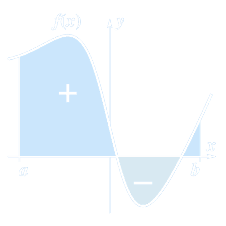
(The definite integral of a function is the signed area of the region bounded by its graph.)
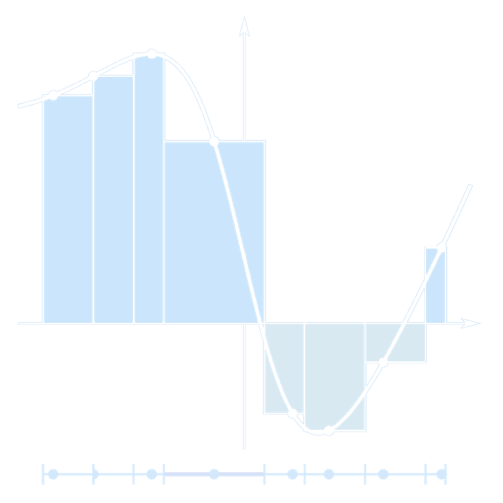
(A Riemann sum of a function \( f \) with respect to a tagged partition.)
The Taylor Formula
Taylor Formula with Peano Remainder: Suppose that $f(x)$ is defined in a neighborhood $(x_0 - \delta, x_0 + \delta) \text{ of } x_0, \text{ and for some } n \in \mathbb{N},$ $f \in D^{(n-1)}(x_0 - \delta, x_0 + \delta), \text{ and } f^{(n)}(x_0) \text{ exists. Then we have}$ $$ \begin{aligned} f(x) &= f(x_0) + f'(x_0)(x - x_0) + \frac{1}{2} f''(x_0)(x - x_0)^2 \\ &\quad + \cdots + \frac{1}{n!} f^{(n)}(x_0)(x - x_0)^n + r_n(x), \end{aligned} $$ where the remainder $r_n(x) \in o((x - x_0)^n)$, as $x \to x_0$.The polynomial $$ p_n(x) = f(x_0) + f'(x_0)(x - x_0) + \frac{1}{2} f''(x_0)(x - x_0)^2 + \cdots + \frac{1}{n!} f^{(n)}(x_0)(x - x_0)^n $$ is called the Taylor polynomial of degree $n$. It can be seen as an approximation of the original function $f$ near $x_0$.
Taylor Formula with Lagrange Remainder: Let $f(x)$ be a function defined on $(a, b)$. If $f \in D^{n+1}(a, b)$, then for any $x$ and $x_0 \in (a, b)$, we have $$ \begin{aligned} f(x) &= f(x_0) + f'(x_0)(x - x_0) + \frac{1}{2} f''(x_0)(x - x_0)^2 \\ &\quad + \cdots + \frac{1}{n!} f^{(n)}(x_0)(x - x_0)^n + r_n(x), \end{aligned} $$ where the remainder $ r_n(x) = \frac{f^{(n+1)}(\zeta)}{(n+1)!} (x - x_0)^{n+1}, $ and $\zeta$ is some number between $x$ and $x_0$ (i.e., $\zeta \in (x, x_0)$ or $(x_0, x)$).
| Common Six Taylor Expansions |
|---|
| \( e^x = 1 + x + \frac{x^2}{2!} + \cdots + \frac{x^n}{n!} + \mathcal{O}(x^n) \) |
| \( \sin x = x - \frac{x^3}{3!} + \frac{x^5}{5!} - \cdots + (-1)^n \frac{x^{2n+1}}{(2n+1)!} + \mathcal{O}(x^{2n+1}) \) |
| \( \cos x = 1 - \frac{x^2}{2!} + \frac{x^4}{4!} - \frac{x^6}{6!} + \cdots + (-1)^n \frac{x^{2n}}{(2n)!} + \mathcal{O}(x^{2n}) \) |
| \( \ln(1+x) = x - \frac{x^2}{2} + \frac{x^3}{3} - \cdots + (-1)^n \frac{x^{n+1}}{n+1} + \mathcal{O}(x^{n+1}) \) |
| \( \frac{1}{1-x} = 1 + x + x^2 + \cdots + x^n + \mathcal{O}(x^n) \) |
| \( (1+x)^m = 1 + mx + \frac{m(m-1)}{2!}x^2 + \cdots + \frac{m(m-1)\cdots(m-n+1)}{n!}x^n + \mathcal{O}(x^n) \) |
[Q] Consider $f(x) = e^x$. Find its Taylor formula near $x_0 = 0$.
[Sol] We have $$ f(x) = f'(x) = f''(x) = \cdots = f^{(n)}(x) = e^x, $$ and $$ f(0) = f'(0) = f''(0) = \cdots = f^{(n)}(0) = 1. $$ $$ \Rightarrow e^x = 1 + x + \frac{x^2}{2!} + \frac{x^3}{3!} + \cdots + \frac{x^n}{n!} + r_n(x), $$ where $ r_n(x) = o(x^n),$ or $r_n(x) = \frac{e^{\eta x}}{(n+1)!} x^{n+1}, $ for some $ \eta \in (0,1)$.
[Q] Consider $f(x) = \sin(x)$. Find its Taylor formula near $x_0 = 0$.
[Sol] $$ \because f^{(k)}(x) = \sin\left(x + \frac{k}{2} \pi\right). $$ $$ \therefore \sin(x) = x - \frac{x^3}{3!} + \frac{x^5}{5!} + \cdots + (-1)^n \frac{x^{2n+1}}{(2n+1)!} + r_{2n+2}(x), $$ where $r_{2n+2}(x) = o(x^{2n+2})$, or $r_{2n+2}(x) = \frac{x^{2n+3}}{(2n+3)!} \sin\left(\eta x + \frac{2n+3}{2} \pi\right)$, for some $\eta \in (0, 1)$.
[Q] Find $\lim_{x \to 0} \frac{\cos(x) - e^{-\frac{x^2}{2}}}{x^4} = \boxed{?}$
[Sol] \begin{align*} \lim_{x \to 0} \frac{\cos(x) - e^{-\frac{x^2}{2}}}{x^4} &= \lim_{x \to 0} \frac{\left[1 - \frac{x^2}{2!} + \frac{x^4}{4!} + o(x^4)\right] - \left[1 + \left(-\frac{x^2}{2}\right) + \frac{1}{2!} \left(-\frac{x^2}{2}\right)^2 + o(x^4)\right]}{x^4} \\ &= \lim_{x \to 0} \frac{-\frac{1}{12}x^4 + o(x^4)}{x^4} \\ &= -\frac{1}{12} \end{align*} The Note 1.1 Mathematical Approximation Methods in An Introduction to Mechanics by Daniel Kleppner and Robert Kolenkow is an excellent text for demonstrating how to apply mathematical approximations in physics.
Areas and Volumes
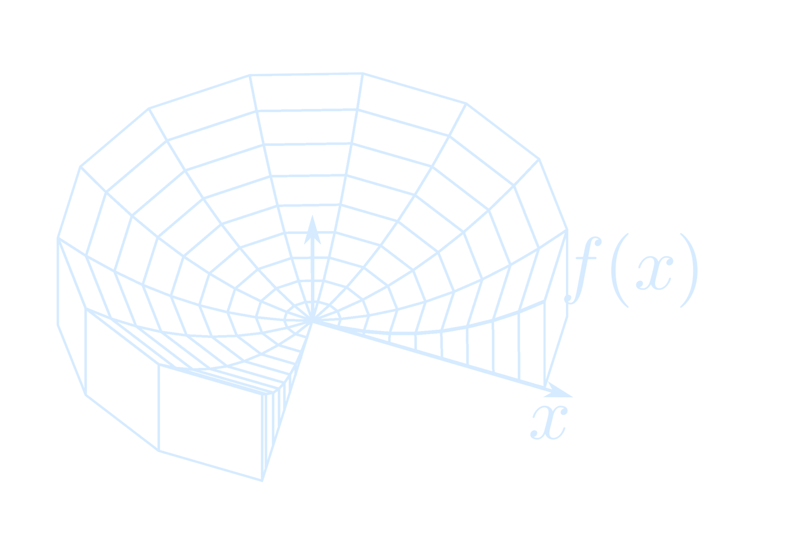
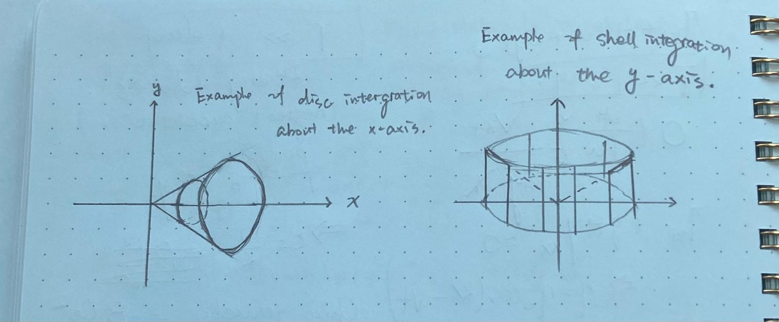
Let $f$ and $g$ be continuous functions whose graphs intersect at the graphical points corresponding to $x = a$ and $x = b$, $a < b$. If $g(x) \leq f(x)$ on $[a, b]$, then the area bounded by $f(x)$ and $g(x)$ is $$ A = \int_a^b [f(x) - g(x)] \, dx $$ Disk method: Disk method, is a means of calculating the volume of a solid of revolution of a solid-state material when integrating along the axis of revolution. This method models the resulting three-dimensional shape as a “stack” of an infinite number of disks of varying radius and infinitesimal thickness.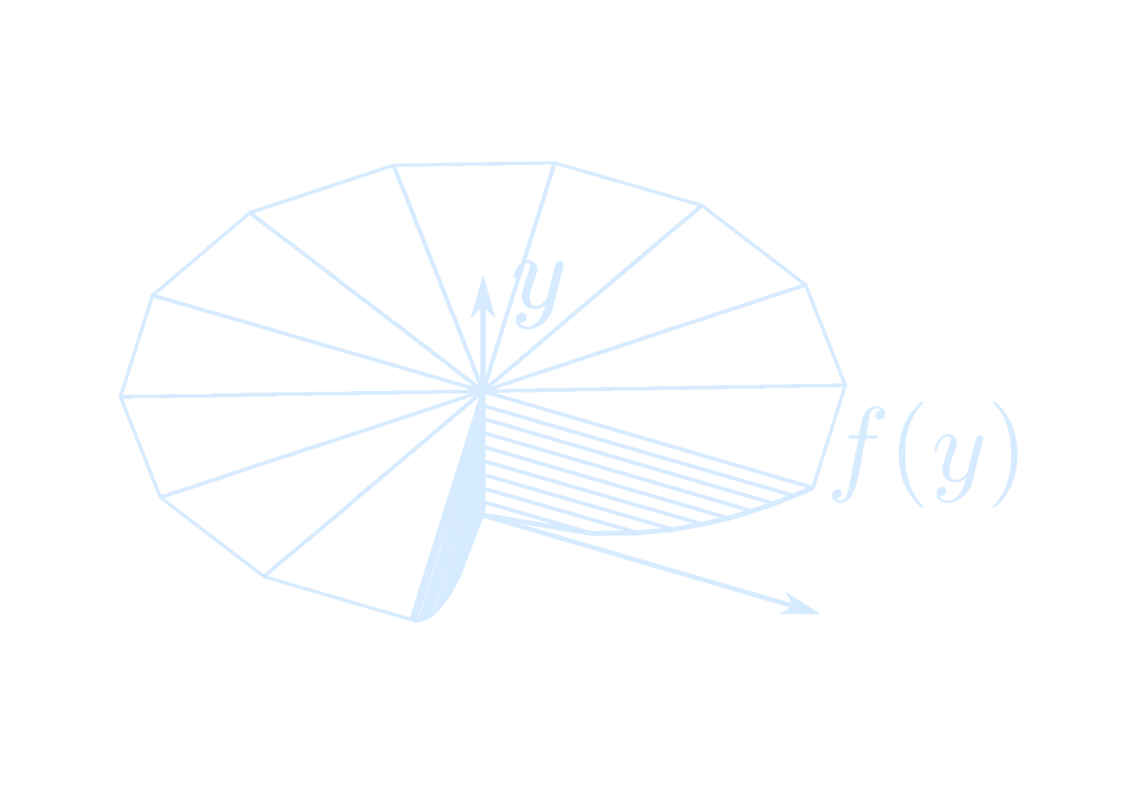
(Disc integration about the y-axis.)
Assume that $x = f(y) \in C[c, d]$ and $f(y) \geq 0$. Then the volume of the solid of revolution obtained by revolving the region between the graph of $f(y)$ on $[c, d]$ about the y-axis is
$$
V = \pi \int_c^d [f(y)]^2 \, dy
$$
Assume that $y = f(x) \in C[a, b]$ and $f(x) \geq 0$. Then the volume of the solid of revolution obtained by revolving the region between the graph of $f(x)$ on $[a, b]$ about the x-axis is
$$
V = \pi \int_a^b [f(x)]^2 \, dx
$$
[Ex] A solid cone is generated by revolving the graph of $y = kx$,
$k > 0$ and $0 \leq x \leq b$, about the x-axis. Its volume is
$$
\begin{aligned}
V &= \pi \int_0^b k^2 x^2 \, dx \\
&= \pi \frac{k^2 b^3}{3}
\end{aligned}
$$
Shell method:Shell method is a means of calculating the volume of a solid of revolution, when integrating along an axis perpendicular to the axis of revolution.
(Shell integration about the y-axis.)
Suppose that $f \in C[a, b]$, $a \geq 0$, and $f(x) \geq 0$. Let $R$ be the plane region bound by $f(x)$, $x = a$, $x = b$, and the x-axis. The volume obtained by rotating $R$ around the y-axis is
$$
V = \int_a^b 2\pi x f(x) \, dx
$$
[Ex] If the region bounded by $y = kx$, $0 \leq x \leq b$ and $x = b$ rotates about the y-axis, then the volume of revolution obtained is
$$
\begin{aligned}
V &= 2\pi \int_0^b x(kx) \, dx \\
&= 2\pi k \frac{b^3}{3}
\end{aligned}
$$
Ordinary Differential Equation
Ordinary Differential Equations (ODEs) has two parts:- Initial Value Problem $$ \frac{d\vec{x}}{dt} = \vec{f}(t, \vec{x}) $$ $$ \vec{x}(t_0) = \vec{x}_0 $$ \(\longleftrightarrow\) Important examples in Dynamical Systems
- Boundary Value Problem
Analytic \(\longleftrightarrow\) Numerical Computational Method
Review of Baby ODE: 1st order scalar differential equation
I.V.P. (Initial Value Problem) $$ \left\{ \begin{aligned} \frac{dx}{dt} &= f(t, x) \\ x(t_0) &= x_0 \end{aligned} \right. \quad \text{where } f : \mathbb{R} \times \mathbb{R} \to \mathbb{R} $$ Separable equations (seperation of variables): $$ \frac{dx}{dt} = g(x) h(t) $$ $$ \int \frac{dx}{g(x)} = \int h(t)\,dt + C $$ $$ \boxed{G(x) = H(t) + C} $$ Express $x$ as a function of $t$ $$ x = x(t), \quad t = \text{time} $$ [Ex]$$ \left\{ \begin{aligned} \frac{dx}{dt} &= ax \\ x(0) &= x_0 \end{aligned} \right. \quad a > 0 $$ $$ x(t) = \text{population of a species at time } t $$ $$ \frac{dx}{dt} = \text{rate of change is proportional to the current population.} $$ $$ \frac{1}{x} \frac{dx}{dt} = a \Rightarrow \frac{dx}{x} = a\,dt $$ $$ \int \frac{dx}{x} = \int a \, dt $$ Integrating both sides: $$ \ln |x| = at + C $$ Exponentiating both sides: $$ x = e^{at + C} = e^C \cdot e^{at} $$ Let $x_0 = e^C$, which is the initial value: $$ x(0) = x_0 $$ $$ \therefore \boxed{x(t) = x_0 e^{at}} $$ [Q] Write $$ \begin{aligned} y'' + 3\sin(zy) + z' &= \cos t \\ z''' + z'' + 3y' + z'y &= t \end{aligned} $$ as an equivalent first order system of differential equations.
[Sol] To write this as a first-order system, define new variables: $$ \begin{aligned} x_1 &= y \\ x_2 &= y' \\ x_3 &= z \\ x_4 &= z' \\ x_5 &= z'' \end{aligned} $$ Now express the system as: $$ \begin{aligned} x_1' &= x_2 \\ x_2' &= \cos t - 3\sin(x_3 x_1) - x_4 \\ x_3' &= x_4 \\ x_4' &= x_5 \\ x_5' &= t - x_5 - 3x_2 - x_4 x_1 \end{aligned} $$ This is the equivalent first-order system of differential equations.
[Q] Show that the solutions $x_1(t), x_2(t)$ of the Lotka–Volterra two species competition model $$ \begin{aligned} \frac{dx_1}{dt} &= r_1 x_1 \left(1 - \frac{x_1}{K_1} \right) - \alpha_1 x_1 x_2 \\ \frac{dx_2}{dt} &= r_2 x_2 \left(1 - \frac{x_2}{K_2} \right) - \alpha_2 x_1 x_2 \\ x_1(0) &> 0,\quad x_2(0) > 0 \end{aligned} $$ are positive and bounded for all $t \geq 0$.
Euler Equations
Differential Equation $$ x^n y^{(n)} + p_1 x^{n-1} y^{(n-1)} + \cdots + p_{n-1} x y' + p_n y = f(x) $$ where $p_1, p_2, \dots, p_n$ are constants. This is called an Euler equation, and its solution method isLet $x = e^t$, i.e., $t = \ln x$, then: $$ \frac{dy}{dx} = \frac{dy}{dt} \cdot \frac{dt}{dx} = \frac{1}{x} \frac{dy}{dt} $$ $$ \frac{d^2 y}{dx^2} = \frac{d}{dx} \left( \frac{1}{x} \frac{dy}{dt} \right) = \frac{1}{x^2} \left( \frac{d^2 y}{dt^2} - \frac{dy}{dt} \right) $$ $$ \frac{d^3 y}{dx^3} = \frac{1}{x^3} \left( \frac{d^3 y}{dt^3} - 3 \frac{d^2 y}{dt^2} + 2 \frac{dy}{dt} \right), \dots $$ Substituting into the original equation transforms the Euler equation into a linear differential equation with constant coefficients.
[Q]The general solution of the Euler equation $ x^2 \frac{d^2 y}{dx^2} + 4x \frac{dy}{dx} + 2y = 0 (x > 0) $ is $ \boxed{ ? }$
[Sol] Let $x = e^t$, then $$ \frac{dy}{dx} = \frac{1}{x} \frac{dy}{dt} = e^{-t} \frac{dy}{dt} \quad \Rightarrow \quad \frac{dy}{dt} = x \frac{dy}{dx}, $$ $$ \frac{d^2y}{dx^2} = \frac{1}{x^2} \left( \frac{d^2y}{dt^2} - \frac{dy}{dt} \right) = \frac{1}{x^2} \left( x^2 \frac{d^2y}{dx^2} + x \frac{dy}{dx} - x \frac{dy}{dx} \right), $$ Substitute into the original equation and simplify get $ \frac{d^2y}{dt^2} + 3\frac{dy}{dt} + 2y = 0 $, solve this equation, the general solution is $$ y = C_1 e^{-t} + C_2 e^{-2t} = \frac{C_1}{x} + \frac{C_2}{x^2} $$ \(\therefore\) The answer is $$ \boxed{y = \frac{C_1}{x} + \frac{C_2}{x^2}} $$
Partial Differential Equation
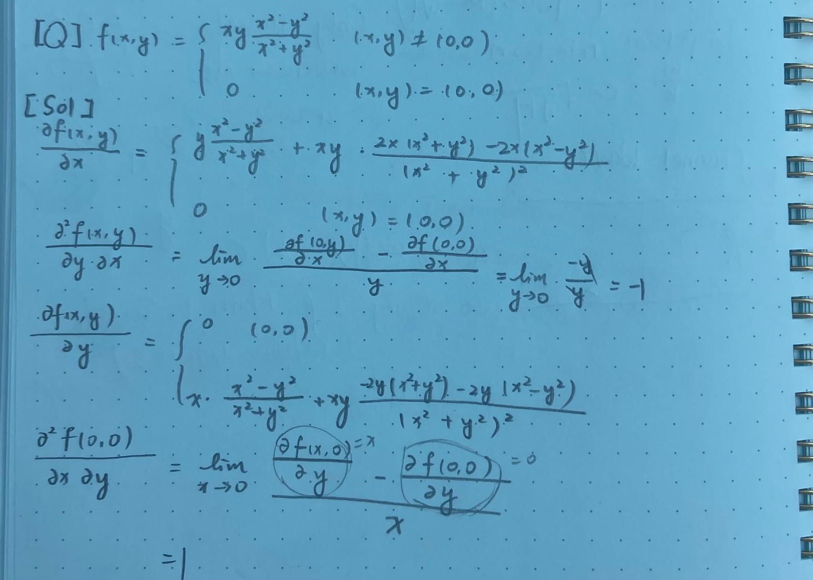
Let the function $z = f(x, y)$ be defined at and near the point $(a, b)$. Consider the function $z = f(x, b)$. The derivative at the point $x = a$ is: $$ \lim_{\Delta x \to 0} \frac{f(a + \Delta x, b) - f(a, b)}{\Delta x}. $$ If this limit exists, then it is called the partial derivative of the function $z = f(x, y)$ at the point $(a, b)$ with respect to $x$. It is denoted as: $$ \frac{\partial f(a, b)}{\partial x}, \quad f_x(a, b), \quad \text{or} \quad \left. \frac{\partial z}{\partial x} \right|_{(a, b)}. $$ $\frac{\partial f(a, b)}{\partial x}$ reflects how the function $f(x, y)$ changes at point $(a, b)$ along the straight line parallel to the $x$-axis. What it depicts is the property along that straight line, and in essence it is the derivative of a single-variable function $ \frac{d}{dx}[f(x, b)] $. Unlike the derivative notation of a single-variable function $\frac{df(x)}{dx}$, the notation for partial derivatives $\frac{\partial f(a,b)}{\partial x}$ is merely a symbol and should not be interpreted as the quotient of two numbers. Unlike single-variable functions, whether the partial derivative of a two-variable function exists at a point has no relation to whether the function is continuous at that point (although there is necessarily a connection).[Q] $z = \sin(xy)$
[Sol] $$ \frac{\partial z}{\partial x} = \cos(xy) \cdot y,\quad \frac{\partial z}{\partial y} = \cos(xy) \cdot x $$ $$ \frac{\partial^2 z}{\partial x^2} = -\sin(xy) \cdot y^2 $$ $$ \frac{\partial^2 z}{\partial y \partial x} = \cos(xy) - xy \cdot \sin(xy) $$ $$ \frac{\partial^2 z}{\partial x \partial y} = \cos(xy) - xy \cdot \sin(xy) $$ $$ \frac{\partial^2 z}{\partial y^2} = -x^2 \cdot \sin(xy) $$ [Q] $ u = \ln(x + y + \delta) $
[Sol] $$ \frac{\partial u}{\partial x} = \frac{1}{x + y + \delta}, \quad \frac{\partial u}{\partial y} = \frac{1}{x + y + \delta} $$ $$ \frac{\partial^2 u}{\partial y \partial x} = -\frac{1}{(x + y + \delta)^2}, \quad \frac{\partial^2 u}{\partial x \partial y} = -\frac{1}{(x + y + \delta)^2} $$
Cylindrical Coordinates
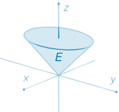
Rectangular coordinates $(x, y, z)$ are related to cylindrical coordinates $(r, \theta, z)$ by $$ \boxed{ \begin{aligned} x &= r \cos(\theta) \\ y &= r \sin(\theta) \\ z &= z \end{aligned} } $$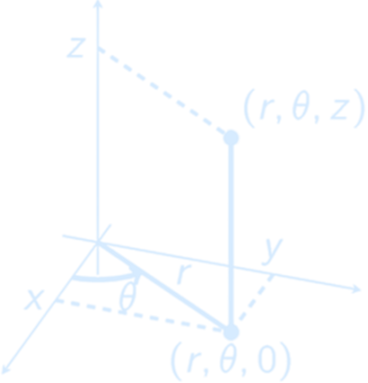 [Ex] Consider region $E$ inside cone
$$
z = \sqrt{x^2 + y^2}
$$
with $0 \leq z \leq 1$. Cone in cylindrical coordinates:
$$
z = \sqrt{x^2 + y^2} = \sqrt{r^2 \cos^2(\theta) + r^2 \sin^2(\theta)} = r.
$$
\(\therefore\) We find
$$
E = \{ (r, \theta, z) \mid 0 \leq r \leq z,\ 0 \leq \theta \leq 2\pi,\ 0 \leq z \leq 1 \}
$$
[Ex] Consider region $E$ inside cone
$$
z = \sqrt{x^2 + y^2}
$$
with $0 \leq z \leq 1$. Cone in cylindrical coordinates:
$$
z = \sqrt{x^2 + y^2} = \sqrt{r^2 \cos^2(\theta) + r^2 \sin^2(\theta)} = r.
$$
\(\therefore\) We find
$$
E = \{ (r, \theta, z) \mid 0 \leq r \leq z,\ 0 \leq \theta \leq 2\pi,\ 0 \leq z \leq 1 \}
$$
 [Ex] The volume element $dV$ in curvilinear coordinates $t^1, t^2, t^3$, as we know, has the form
$$
dV = \sqrt{\det g_{ij}(t)} \, dt^1 \wedge dt^2 \wedge dt^3.
$$
For a triorthogonal system,
$$
dV = \sqrt{E_1 E_2 E_3(t)} \, dt^1 \wedge dt^2 \wedge dt^3.
$$
In particular, in Cartesian, cylindrical, and spherical coordinates, respectively, we obtain
$$
\begin{aligned}
dV &= dx \wedge dy \wedge dz = \\
&= r \, dr \wedge d\varphi \wedge dz = \\
&= R^2 \cos \theta \, dR \wedge d\varphi \wedge d\theta.
\end{aligned}
$$
What has just been said enables us to write the form $\omega^3_\rho = \rho \, dV$ in different curvilinear coordinate systems.
Repeated equal signs represent a continuation of equalities across different coordinate systems, and show how the same geometric object (volume form $dV$) takes different analytic forms in different systems.
[Ex] The volume element $dV$ in curvilinear coordinates $t^1, t^2, t^3$, as we know, has the form
$$
dV = \sqrt{\det g_{ij}(t)} \, dt^1 \wedge dt^2 \wedge dt^3.
$$
For a triorthogonal system,
$$
dV = \sqrt{E_1 E_2 E_3(t)} \, dt^1 \wedge dt^2 \wedge dt^3.
$$
In particular, in Cartesian, cylindrical, and spherical coordinates, respectively, we obtain
$$
\begin{aligned}
dV &= dx \wedge dy \wedge dz = \\
&= r \, dr \wedge d\varphi \wedge dz = \\
&= R^2 \cos \theta \, dR \wedge d\varphi \wedge d\theta.
\end{aligned}
$$
What has just been said enables us to write the form $\omega^3_\rho = \rho \, dV$ in different curvilinear coordinate systems.
Repeated equal signs represent a continuation of equalities across different coordinate systems, and show how the same geometric object (volume form $dV$) takes different analytic forms in different systems.[Q] In cylindrical coordinates $(r, \varphi, z)$ the function $f$ has the form $\ln \frac{1}{r}$. Write the field $\mathbf{A} = \nabla f$ in
- Cartesian coordinates
- Cylindrical coordinates
- Spherical coordinates
- Find curl $\mathbf{A}$ and div $\mathbf{A}$
Polar Coordinates
Our new coordinate system is based on the cylindrical coordinate system. The $z$ axis of the cylindrical system is identical to that of the cartesian system. However, position in the $xy$ plane is described by distance $r$ from the $z$ axis and the angle $\theta$ that $r$ makes with the $x$ axis. These coordinates are shown in the sketch. We see that $$ r = \sqrt{x^2 + y^2} $$ $$ \theta = \arctan\left(\frac{y}{x}\right) $$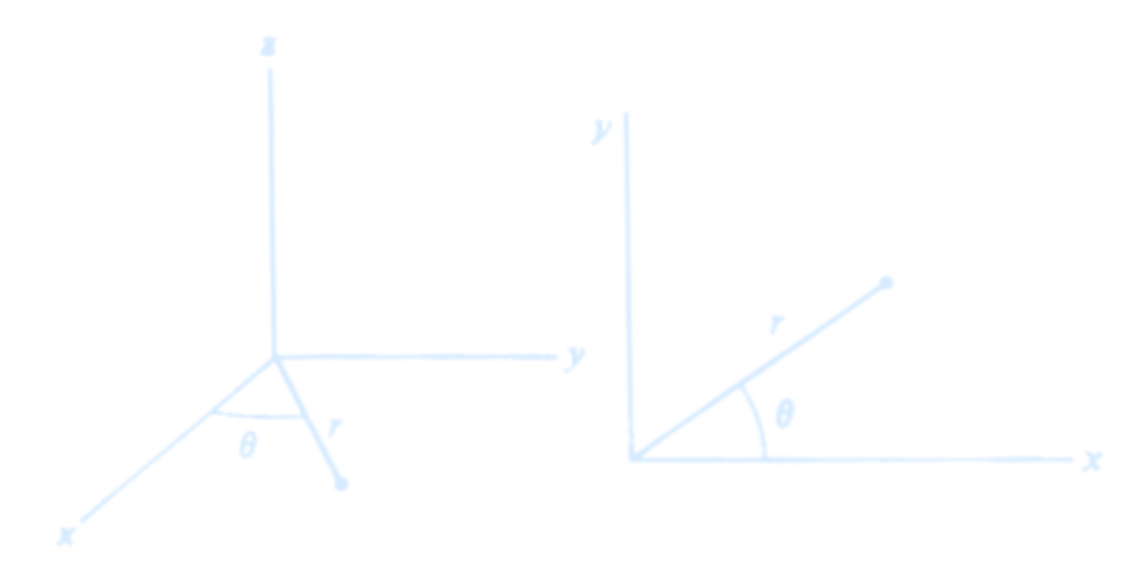 Since we shall be concerned primarily with motion in a plane, we neglect the $z$ axis and restrict our discussion to two dimensions. The coordinates $r$ and $\theta$ are called plane polar coordinates.
The contrast between cartesian and plane polar coordinates is readily seen by comparing drawings of constant coordinate lines for the two systems.
The lines of constant $x$ and of constant $y$ are straight and perpendicular to each other.
Lines of constant $\theta$ are also straight, directed radially outward from the origin.
In contrast, lines of constant $r$ are circles concentric to the origin.
Since we shall be concerned primarily with motion in a plane, we neglect the $z$ axis and restrict our discussion to two dimensions. The coordinates $r$ and $\theta$ are called plane polar coordinates.
The contrast between cartesian and plane polar coordinates is readily seen by comparing drawings of constant coordinate lines for the two systems.
The lines of constant $x$ and of constant $y$ are straight and perpendicular to each other.
Lines of constant $\theta$ are also straight, directed radially outward from the origin.
In contrast, lines of constant $r$ are circles concentric to the origin.Note: the lines of constant $\theta$ and constant $r$ are perpendicular wherever they intersect.
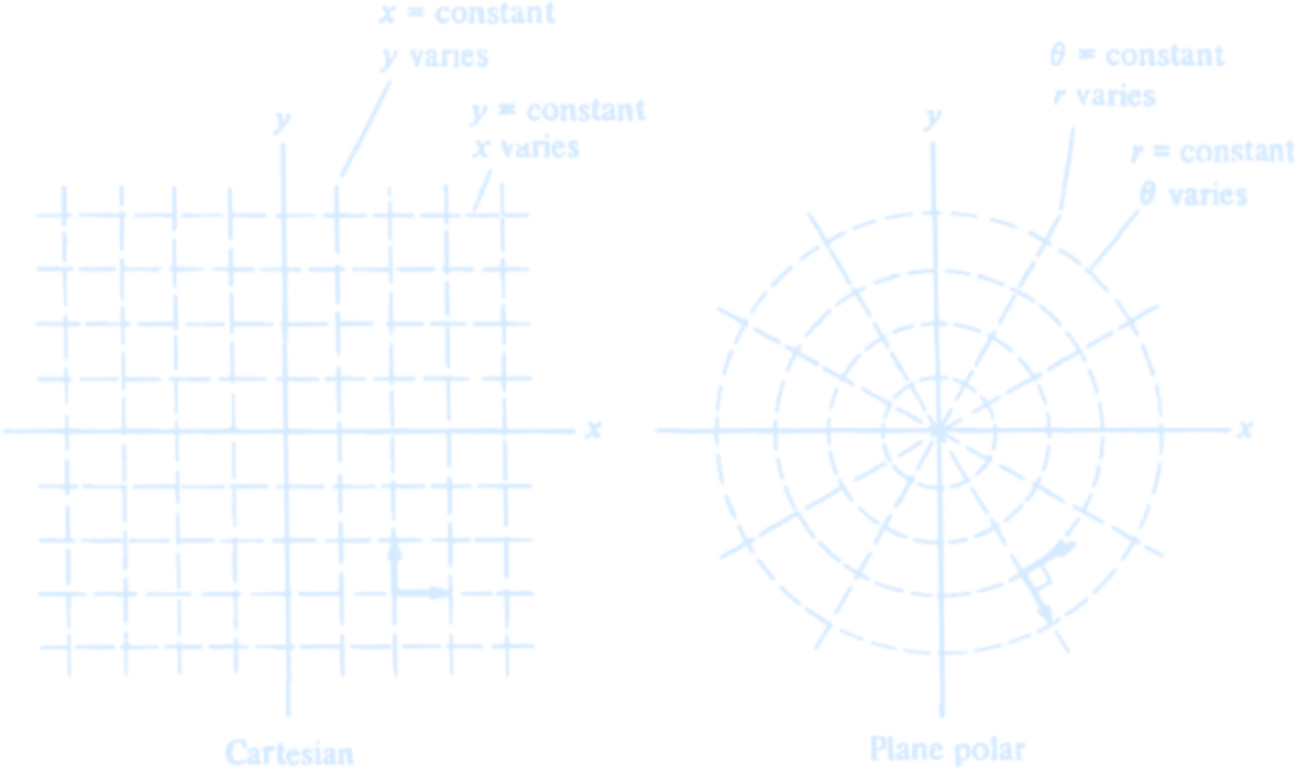
(Credit: An Introduction to Mechanics by Daniel Kleppner & Robert Kolenkow.)
Spherical Coordinates
 The usual cartesian coordinate system associated with the Earth is specified as follows:
- The origin is the center of the Earth.
- The z-axis is the rotational axis. It pierces the Earth at the poles and its positive direction is towards the north pole. The Earth rotates in the positive direction around this z-axis: when you lay your right hand on the globe such that the thumb shows to the north pole, then the Earth rotates in the direction of the fingers ("the rule of the right hand").
- Great circles passing through the poles are called meridians. The Prime Meridian passes through Royal Observatory in Greenwich (London).
- The plane that is orthogonal to the z-axis is the equatorial plane and the great circle that is located in this plane is the equator.
- The x-axis points towards the intersection of the prime meridian with the equator.
- The y-axis is in the equator plane, it is orthogonal to the x-axis and oriented such that the coordinates build a right-handed system. When the fingers of the right hand go from the x- to the y-axis then the thumb shows in the direction of the z-axis.
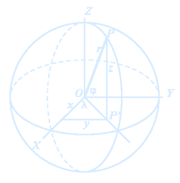
Points on the Earth are usually specified in the spherical coordinate system. The spherical coordinates of an arbitrary cartesian point $P(x, y, z)$ are:
- The latitude $\varphi$ which is the angle between $OP$ and the equator.
- The longitude $\lambda$ which is the angle between the prime meridian and the meridian passing through $OP$.
- The radius $r$ which is the distance of $P$ from the origin.
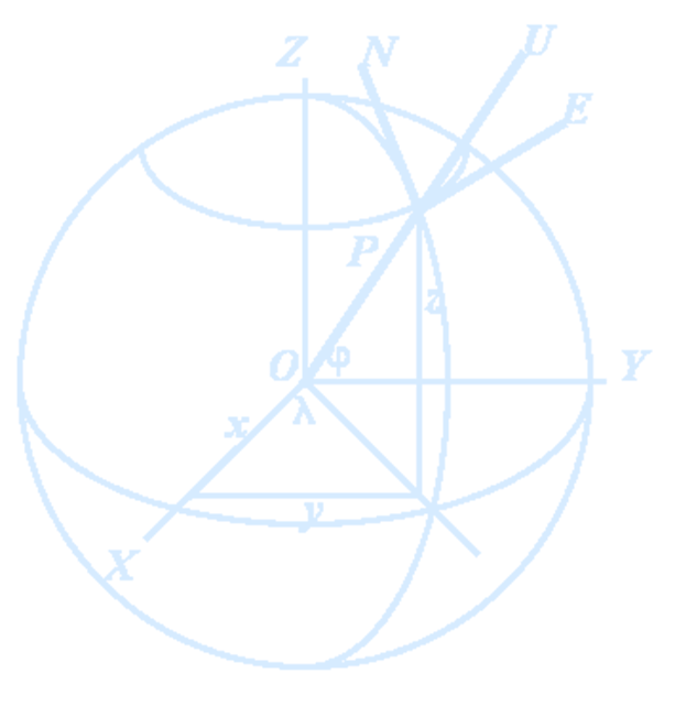 An East-North-Up (ENU) system uses the Cartesian coordinates (xEast,yNorth,zUp) to represent position relative to a local origin.
The ENU coordinate system is a local system specific to any point $P$ on the Earth. It is formed from a plane tangent to the Earth's surface at the point $P$. In this plane:
An East-North-Up (ENU) system uses the Cartesian coordinates (xEast,yNorth,zUp) to represent position relative to a local origin.
The ENU coordinate system is a local system specific to any point $P$ on the Earth. It is formed from a plane tangent to the Earth's surface at the point $P$. In this plane:
- The unit vector $\mathbf{E}$ points to the East
- The unit vector $\mathbf{N}$ points to the North
- The unit vector $\mathbf{U}$ points Up, i.e., is orthogonal to the tangent plane.
[Ex] In particular, for Cartesian, cylindrical, and spherical coordinates, we obtain respectively: $$ \begin{aligned} \Delta f &= \frac{\partial^2 f}{\partial x^2} + \frac{\partial^2 f}{\partial y^2} + \frac{\partial^2 f}{\partial z^2} = \\ &= \frac{1}{r} \frac{\partial}{\partial r} \left( r \frac{\partial f}{\partial r} \right) + \frac{1}{r^2} \frac{\partial^2 f}{\partial \varphi^2} + \frac{\partial^2 f}{\partial z^2} = \\ &= \frac{1}{R^2} \frac{\partial}{\partial R} \left( R^2 \frac{\partial f}{\partial R} \right) + \frac{1}{R^2 \cos^2 \theta} \frac{\partial^2 f}{\partial \varphi^2} + \frac{1}{R^2 \cos \theta} \frac{\partial}{\partial \theta} \left( \cos \theta \frac{\partial f}{\partial \theta} \right) \end{aligned} $$
The Gradient
Almost any book with mathematical problems and even any textbook of mathematical analysis states something like the following. “Children, remember”: We call the gradient of a function $U(u, x, z)$ the vector $$ \text{grad } U := \left( \frac{\partial U}{\partial x}, \frac{\partial U}{\partial y}, \frac{\partial U}{\partial z} \right) $$ The curl of a vector field $\mathbf{A} = (P, Q, R)(x, y, z)$ is the vector $$ \text{curl } \mathbf{A} := \left( \frac{\partial R}{\partial y} - \frac{\partial Q}{\partial z}, \frac{\partial P}{\partial z} - \frac{\partial R}{\partial x}, \frac{\partial Q}{\partial x} - \frac{\partial P}{\partial y} \right) $$ The divergence of a vector field $\mathbf{B} = (P, Q, R)(x, y, z)$ is the function $$ \text{div } \mathbf{B} := \frac{\partial P}{\partial x} + \frac{\partial Q}{\partial y} + \frac{\partial R}{\partial z} $$ The fact that this is true only in Cartesian coordinates is not usually discussed, as well as what should be done if the coordinate system is different. This is understandable, since the very formulation of this problem already requires some suitable definition of these objects.Divergence and Curl
[Q]The operators grad, curl, and div and the algebraic operations. Verify the following relations:- for grad:
- (a) $\nabla(f + g) = \nabla f + \nabla g$
- (b) $\nabla(f \cdot g) = f \nabla g + g \nabla f$
- (c) $\nabla(\mathbf{A} \cdot \mathbf{B}) = (\mathbf{B} \cdot \nabla)\mathbf{A} + (\mathbf{A} \cdot \nabla)\mathbf{B} + \mathbf{B} \times (\nabla \times \mathbf{A}) + \mathbf{A} \times (\nabla \times \mathbf{B})$
- (d) $\nabla\left( \frac{1}{2} A^2 \right) = (\mathbf{A} \cdot \nabla)\mathbf{A} + \mathbf{A} \times (\nabla \times \mathbf{A})$
- for curl:
- (e) $\nabla \times (f \mathbf{A}) = f \nabla \times \mathbf{A} + \nabla f \times \mathbf{A}$
- (f) $\nabla \times (\mathbf{A} \times \mathbf{B}) = (\mathbf{B} \cdot \nabla)\mathbf{A} - (\mathbf{A} \cdot \nabla)\mathbf{B} + (\nabla \cdot \mathbf{B})\mathbf{A} - (\nabla \cdot \mathbf{A})\mathbf{B}$
- for div:
- (g) $\nabla \cdot (f \mathbf{A}) = \nabla f \cdot \mathbf{A} + f \nabla \cdot \mathbf{A}$
- (h) $\nabla \cdot (\mathbf{A} \times \mathbf{B}) = \mathbf{B} \cdot (\nabla \times \mathbf{A}) - \mathbf{A} \cdot (\nabla \times \mathbf{B})$
Laplace Operator
If $\mathbf{a}$ is the gradient of a scalar function $\nabla f$, its divergence is called the Laplacian of $f$. $$ \nabla^2 f = \nabla \cdot \nabla f = \Delta f $$ A function that satisfied Laplace’s equation $\nabla^2 f = 0$ is called a potential function.- For a scalar function $f$: $$ \nabla^2 f = \frac{\partial^2 f}{\partial x^2} + \frac{\partial^2 f}{\partial y^2} + \frac{\partial^2 f}{\partial z^2} $$ $$ \nabla \cdot \nabla f = \nabla \cdot \left( \frac{\partial f}{\partial x} \mathbf{i} + \frac{\partial f}{\partial y} \mathbf{j} + \frac{\partial f}{\partial z} \mathbf{k} \right) $$ $$ = \frac{\partial}{\partial x} \left( \frac{\partial f}{\partial x} \right) + \frac{\partial}{\partial y} \left( \frac{\partial f}{\partial y} \right) + \frac{\partial}{\partial z} \left( \frac{\partial f}{\partial z} \right) $$ $$ = \frac{\partial^2 f}{\partial x^2} + \frac{\partial^2 f}{\partial y^2} + \frac{\partial^2 f}{\partial z^2} = \nabla^2 f $$ [Ex] The Laplacian of the scalar field $f(x, y, z) = xy^2 + z^3$ is $$ \nabla^2 f(x, y, z) = \frac{\partial^2 f}{\partial x^2} + \frac{\partial^2 f}{\partial y^2} + \frac{\partial^2 f}{\partial z^2} $$ $$ = \frac{\partial^2}{\partial x^2} (xy^2 + z^3) + \frac{\partial^2}{\partial y^2} (xy^2 + z^3) + \frac{\partial^2}{\partial z^2} (xy^2 + z^3) $$ $$ = \frac{\partial}{\partial x} (y^2 + 0) + \frac{\partial}{\partial y} (2xy + 0) + \frac{\partial}{\partial z} (0 + 3z^2) $$ $$ = 0 + 2x + 6z = 2x + 6z $$
- For a vector field $\vec{f}$, apply the Laplace operator to each component of the vector field individually. That is: $$ \nabla^2 \vec{f} = \left( \nabla^2 f_x, \nabla^2 f_y, \nabla^2 f_z \right) $$ In addition, there is a commonly used equation: $$ \nabla^2 \vec{f} = \nabla (\nabla \cdot \vec{f}) - \nabla \times (\nabla \times \vec{f}) $$ [Ex] The Laplacian of $ \mathbf{F}(x, y, z) = 3z^2\mathbf{i} + xyz\mathbf{j} + x^2z^2\mathbf{k} $ is: $$ \nabla^2 \mathbf{F}(x, y, z) = \nabla^2 (3z^2)\mathbf{i} + \nabla^2 (xyz)\mathbf{j} + \nabla^2 (x^2z^2)\mathbf{k} $$ Calculating the components in turn we find: $$ \nabla^2 (3z^2) = \frac{\partial^2}{\partial x^2}(3z^2) + \frac{\partial^2}{\partial y^2}(3z^2) + \frac{\partial^2}{\partial z^2}(3z^2) = 0 + 0 + 6 = 6 $$ $$ \nabla^2 (xyz) = \frac{\partial^2}{\partial x^2}(xyz) + \frac{\partial^2}{\partial y^2}(xyz) + \frac{\partial^2}{\partial z^2}(xyz) = 0 + 0 + 0 = 0 $$ $$ \nabla^2 (x^2z^2) = \frac{\partial^2}{\partial x^2}(x^2z^2) + \frac{\partial^2}{\partial y^2}(x^2z^2) + \frac{\partial^2}{\partial z^2}(x^2z^2) = 2z^2 + 0 + 2x^2 $$ \(\therefore\) The Laplacian of $\mathbf{F}$ is: $$ \nabla^2 \mathbf{F} = 6\mathbf{i} + 0\mathbf{j} + (2z^2 + 2x^2)\mathbf{k} = 6\mathbf{i} + 2(x^2 + z^2)\mathbf{k} $$
So why is the divergence of the gradient of a scalar field important? My personal understanding is that because the divergence of the gradient of a scalar field represents the “driving force” (or potential “trend”) within the field, and this “driving force” can reveal how the system changes from the inside. The spatial temperature field $T(x, y, z)$ is a scalar field, and its gradient field $\nabla T$ determines the spatial heat flux (heat density flux) vector field $\vec{q}$. At any given point in space, the magnitude of the heat flux is proportional to the magnitude of the gradient (here we assume the material is isotropic). The heat flux vector points in the opposite direction of the temperature gradient. In mathematical terms, it is written as: $$ \vec{q} = -k \nabla T $$ where $k > 0$. Taking the divergence of the above heat flux field (essentially taking the divergence of the temperature gradient field) gives the heat source/sink at a point in space: If the divergence is positive, heat flows out — it’s a heat source; If the divergence is negative, heat flows in — it’s a heat sink. You may have seen the heat conduction equation: $$ \frac{\partial^2 T}{\partial x^2} + \frac{\partial^2 T}{\partial y^2} + \frac{\partial^2 T}{\partial z^2} = 0 $$ (this is the standard Laplace equation described in Cartesian coordinates). Translated into plain language, this equation says: There is no heat source in the space!
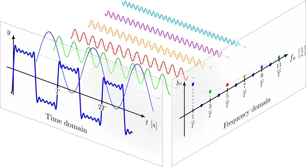
Fourier Series
Fourier Series in Trigonometric Form for Periodic Signals: Trigonometric function set $$ \left\{ 1, \cos(n\Omega t), \sin(n\Omega t), \quad n = 1, 2, \ldots \right\} $$ Let the periodic signal be $f(t)$, with period $T$, and angular frequency $$ \Omega = \frac{2\pi}{T} $$ When the Dirichlet conditions are satisfied, the signal can be expanded as a Fourier series in trigonometric form: $$ f(t) = \underbrace{\frac{a_0}{2}}_{\substack{\text{Direct Current} \\ \text{(DC component)}}} + \underbrace{\sum_{n=1}^{\infty} a_n \cos(n\Omega t)}_{\text{n-th cosine harmonic}} + \underbrace{\sum_{n=1}^{\infty} b_n \sin(n\Omega t)}_{\text{n-th sine harmonic}} $$ The coefficients $a_n$ and $b_n$ are called Fourier coefficients.- DC component: $ \frac{a_0}{2} = \frac{1}{T} \int_{-\frac{T}{2}}^{\frac{T}{2}} f(t) \, dt $
- Cosine Harmonic Coefficients: $ a_n = \frac{2}{T} \int_{-\frac{T}{2}}^{\frac{T}{2}} f(t) \cos(n\Omega t) \, dt $
- Sine Harmonic Coefficients: $ b_n = \frac{2}{T} \int_{-\frac{T}{2}}^{\frac{T}{2}} f(t) \sin(n\Omega t) \, dt $
- Condition 1: Within one period, the function is either continuous or has only a finite number of first-kind discontinuities (i.e., jump discontinuities).
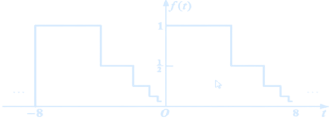 (Counterexample)
 - Condition 2: Within one period, the function must have only a finite number of maxima and minima
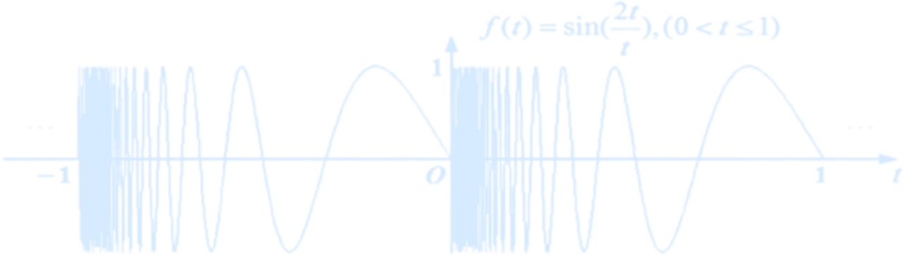 (Counterexample)
 - Condition 3: Within one period, the function must be absolutely integrable.
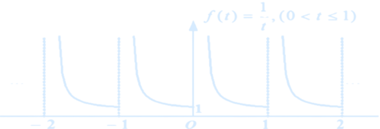 (Counterexample)
- $\frac{A_0}{2}$: DC component
- $A_1 \cos(\Omega t + \varphi_1)$: Called the fundamental wave or first harmonic, its angular frequency is the same as the original signal.
- $A_2 \cos(2\Omega t + \varphi_2)$: Called the second harmonic
- ⋯
- $A_n \cos(n\Omega t + \varphi_n)$: Called the n-th harmonic
[Q] Expand the square wave signal $f(t)$ shown in the figure as a Fourier series.
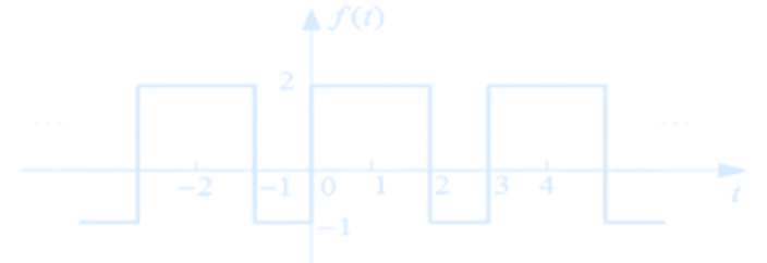 [Sol] To calculate the cosine coefficients:
$$
a_n = \frac{2}{T} \int_{-\frac{T}{2}}^{\frac{T}{2}} f(t) \cos(n\Omega t)\,dt
$$
Break the integral over two intervals:
$$
= \frac{2}{T} \int_{-\frac{T}{2}}^{0} (-1) \cdot \cos(n\Omega t)\,dt + \frac{2}{T} \int_{0}^{\frac{T}{2}} 1 \cdot \cos(n\Omega t)\,dt
$$
$$
= \frac{2}{T} \cdot \frac{1}{n\Omega} \left[ -\sin(n\Omega t) \right]_{-\frac{T}{2}}^{0} + \frac{2}{T} \cdot \frac{1}{n\Omega} \left[ \sin(n\Omega t) \right]_{0}^{\frac{T}{2}}
$$
Considering that $\Omega = \frac{2\pi}{T}$, obtain:
$
\boxed{a_n = 0}
$
[Sol] To calculate the cosine coefficients:
$$
a_n = \frac{2}{T} \int_{-\frac{T}{2}}^{\frac{T}{2}} f(t) \cos(n\Omega t)\,dt
$$
Break the integral over two intervals:
$$
= \frac{2}{T} \int_{-\frac{T}{2}}^{0} (-1) \cdot \cos(n\Omega t)\,dt + \frac{2}{T} \int_{0}^{\frac{T}{2}} 1 \cdot \cos(n\Omega t)\,dt
$$
$$
= \frac{2}{T} \cdot \frac{1}{n\Omega} \left[ -\sin(n\Omega t) \right]_{-\frac{T}{2}}^{0} + \frac{2}{T} \cdot \frac{1}{n\Omega} \left[ \sin(n\Omega t) \right]_{0}^{\frac{T}{2}}
$$
Considering that $\Omega = \frac{2\pi}{T}$, obtain:
$
\boxed{a_n = 0}
$To compute the sine coefficients: $$ b_n = \frac{2}{T} \int_{-\frac{T}{2}}^{\frac{T}{2}} f(t) \sin(n\Omega t)\,dt = \frac{2}{T} \int_{-\frac{T}{2}}^{0} (-1)\sin(n\Omega t)\,dt + \frac{2}{T} \int_{0}^{\frac{T}{2}} 1 \cdot \sin(n\Omega t)\,dt $$ $$ = \frac{2}{T} \cdot \frac{1}{n\Omega} \left[ -\cos(n\Omega t) \right]_{-\frac{T}{2}}^{0} + \frac{2}{T} \cdot \frac{1}{n\Omega} \left[ -\cos(n\Omega t) \right]_{0}^{\frac{T}{2}} $$ $$ = \frac{2}{T} \cdot \frac{1}{n\Omega} \left( [1 - \cos(n\Omega T/2)] + [1 - \cos(n\Omega T/2)] \right) $$ $$ = \frac{2}{T} \cdot \frac{1}{n\Omega} \cdot 2[1 - \cos(n\pi)] = \frac{4}{nT\Omega}[1 - \cos(n\pi)] $$ Since $\Omega = \frac{2\pi}{T}$, we get: $$ b_n = \frac{2}{n\pi}[1 - \cos(n\pi)] = \begin{cases} 0, & n = 2, 4, 6, \dots \\ \frac{4}{n\pi}, & n = 1, 3, 5, \dots \end{cases} $$ The Fourier series expansion of the signal is: $$ f(t) = \frac{a_0}{2} + \sum_{n=1}^{\infty} a_n \cos(n\Omega t) + \sum_{n=1}^{\infty} b_n \sin(n\Omega t) $$ $$ = \underbrace{0}_{\text{DC}} + \underbrace{\frac{4}{\pi} \sin(\Omega t)}_{\text{Fundamental}} + \underbrace{\frac{4}{3\pi} \sin(3\Omega t)}_{\text{3rd harmonic}} + \cdots + \underbrace{\frac{4}{n\pi} \sin(n\Omega t)}_{\text{n-th harmonic}}, \quad n = 1, 3, 5, \dots $$
import numpy as np
import matplotlib.pyplot as plt

T = 2
A = 1
t = np.linspace(0, 2, 1000)

# Function to compute partial sum
def square_wave_sum(t, max_n):
    result = np.zeros_like(t)
    for n in range(1, max_n+1, 2):
        result += (4*A)/(np.pi*n) * np.sin(2*np.pi*n*t/T)
    return result

# Harmonics for each subplot
harmonic_limits = [1, 3, 5, 7, 99, 999]
titles = [
    "(a) Fundamental (1st harmonic)",
    "(b) 1st & 3rd harmonics",
    "(c) 1st, 3rd & 5th harmonics",
    "(d) 1st, 3rd, 5th & 7th harmonics",
    "(e) 1st, 3rd, ... up to 99th harmonics",
    "(f) 1st, 3rd, ... up to 999th harmonics (Gibbs phenomenon)"
]

fig, axs = plt.subplots(2, 3, figsize=(16, 9), dpi=300)
axs = axs.flatten()

for i, (ax, N, title) in enumerate(zip(axs, harmonic_limits, titles)):
    y = square_wave_sum(t, N)
    ax.plot(t, y, color='#7DCDF4')
    ax.set_title(title, fontsize=12)
    ax.set_xlim(0, 2)
    ax.set_ylim(-1.5, 1.5)
    ax.grid(True)
    ax.set_xlabel('t [s]')
    ax.set_ylabel('Amplitude')

plt.tight_layout()
plt.show()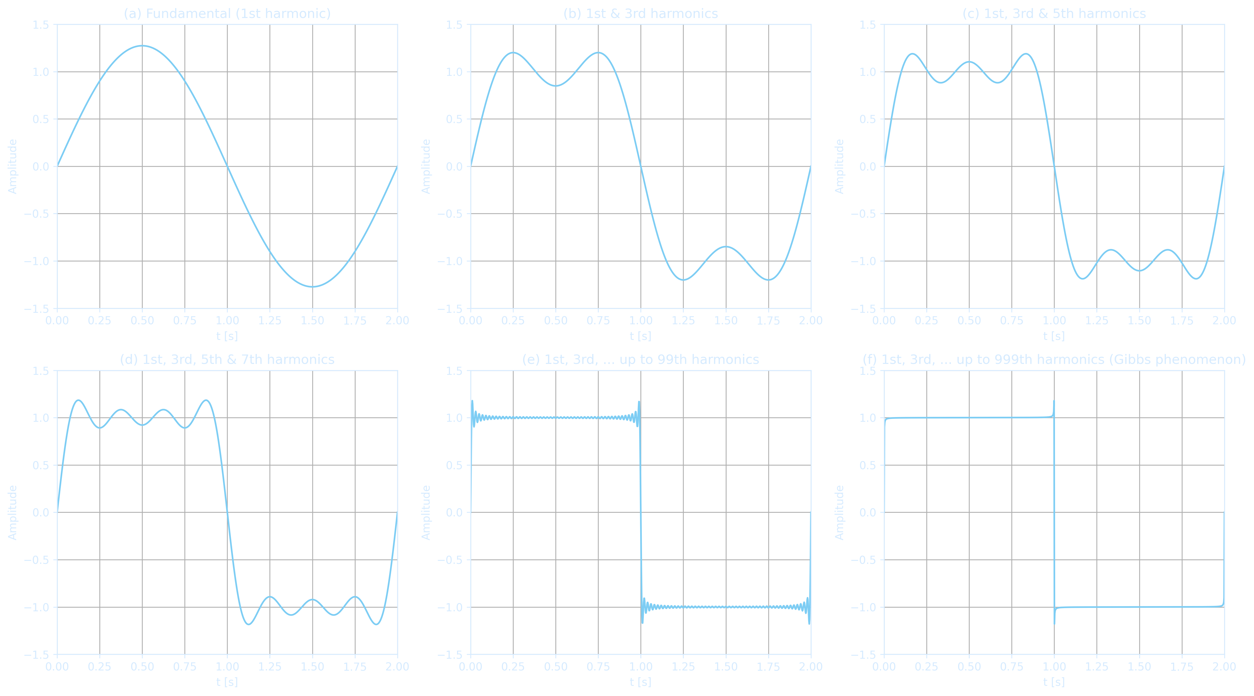
Exponential Form of Fourier Series
The trigonometric form of the Fourier series is conceptually clear but computationally inconvenient, so we often use the exponential form of the Fourier series. \begin{align*} f(t) &= \frac{A_0}{2} + \underbrace{\sum_{n=1}^{\infty} A_n \cos(n\Omega t + \varphi_n)}_{\text{Trigonometric form of the Fourier series}} \\ &= \frac{A_0}{2} + \underbrace{\sum_{n=1}^{\infty} \frac{A_n}{2} \left[ e^{j(n\Omega t + \varphi_n)} + e^{-j(n\Omega t + \varphi_n)} \right]}_{\text{Using Euler's formula}} \\ &= \frac{A_0}{2} + \frac{1}{2} \sum_{n=1}^{\infty} A_n e^{j\varphi_n} e^{jn\Omega t} \boxed{- \underbrace{\frac{1}{2} \sum_{n=1}^{\infty} A_n e^{-j\varphi_n} e^{-jn\Omega t}}_{ \begin{aligned} &\begin{cases} -n \rightarrow n \\ A_{-n} = A_n \\ \varphi_{-n} = -\varphi_n \end{cases} \end{aligned} }} \\ &= \frac{A_0}{2} + \frac{1}{2} \sum_{n=1}^{\infty} A_n e^{j\varphi_n} e^{jn\Omega t} \boxed{+ \frac{1}{2} \sum_{n=-1}^{-\infty} A_n e^{j\varphi_n} e^{jn\Omega t}} \\ \end{align*} Let the complex number $$ \frac{1}{2} A_n e^{j\varphi_n} = |F_n| e^{j\varphi_n} = F_n $$ be called the complex Fourier coefficient, or simply the Fourier coefficient. $$ F_n = \frac{1}{2} A_n e^{j\varphi_n} = \frac{1}{2} (A_n \cos\varphi_n + j A_n \sin\varphi_n) = \frac{1}{2} (a_n - j b_n) $$ $$ = \frac{1}{T} \int_{-\frac{T}{2}}^{\frac{T}{2}} f(t) \cos(n\Omega t) \, \mathrm{d}t - j \frac{1}{T} \int_{-\frac{T}{2}}^{\frac{T}{2}} f(t) \sin(n\Omega t) \, \mathrm{d}t $$ [Q]Find the exponential form of the Fourier series for the periodic signal shown in the figure.
[Sol]Given that $f(t)$ has a period $T = 3$, and $\Omega = \frac{2\pi}{T} = \frac{2\pi}{3}$, it is a periodic signal with period 3. The exponential Fourier coefficient is: $$ \begin{aligned} F_n &= \frac{1}{T} \int_0^T f(t)e^{-jn\Omega t} \, dt \\ &= \frac{1}{3} \left[ \int_0^2 2e^{-jn\Omega t} \, dt - \int_2^3 e^{-jn\Omega t} \, dt \right] \\ &= \frac{2}{j3n\Omega} \left[1 - e^{-j2n\Omega}\right] + \frac{1}{j3n\Omega} \left[e^{-j3n\Omega} - e^{-j2n\Omega} \right] \\ &= \frac{2 - 3e^{-j2n\Omega} + e^{-j3n\Omega}}{j3n\Omega} \\ &= \frac{2 - 3e^{-j\frac{4\pi}{3}n} + e^{-j2\pi n}}{j2\pi n} \\ &= \frac{3}{j2\pi n} \left(1 - e^{-j\frac{4\pi}{3}n}\right) \end{aligned} $$ \(\therefore\) The exponential form of the Fourier series is: $$ f(t) = \sum_{n=-\infty}^{\infty} F_n e^{jn\Omega t} = \sum_{n=-\infty}^{\infty} \frac{3}{j2\pi n} \left(1 - e^{-j\frac{4\pi}{3}n}\right) e^{jn\Omega t} $$
| Expression | Description |
|---|---|
| \( f(t) = \sum_{n=-\infty}^{\infty} F_n e^{jn\Omega t} \) | Exponential Form Fourier Series |
| \( F_n = \frac{1}{T} \int_{-\frac{T}{2}}^{\frac{T}{2}} f(t) e^{-jn\Omega t} \, dt \) | Complex Fourier Coefficient |
Relationship Between Two Fourier Series Forms
| Expression | Type |
|---|---|
| \( f(t) = \frac{a_0}{2} + \sum_{n=1}^{\infty} a_n \cos(n\Omega t) + \sum_{n=1}^{\infty} b_n \sin(n\Omega t) \) | Trigonometric Form Fourier Series |
| \( = \frac{A_0}{2} + \sum_{n=1}^{\infty} A_n \cos(n\Omega t + \varphi_n) \) | |
| \( f(t) = \sum_{n=-\infty}^{\infty} F_n e^{jn\Omega t} \) | Exponential Form Fourier Series |
| \( F_n = |F_n| e^{j\varphi_n} = \frac{1}{2} A_n e^{j\varphi_n} = \frac{1}{2}(a_n - jb_n) \) |
The Fourier Transform
$$ F(j\omega) = \int_{-\infty}^{\infty} f(t) e^{-j\omega t} \, dt $$ $F(j\omega)$ is called the Fourier transform of $f(t)$. $F(j\omega)$ is generally a complex function, expressed as: $$ F(j\omega) = |F(j\omega)| e^{j\varphi(\omega)} $$- $|F(j\omega)| \sim \omega$ — this is the amplitude spectrum, and is an even function of frequency $\omega$.
- $\varphi(\omega) \sim \omega$ — this is the phase spectrum, and it is an odd function of frequency $\omega$.
When $T \to \infty$:
- $\Omega \to d\omega$ (differential element)
- $n\Omega \to \omega$ (discrete $\to$ continuous)
- $\lim_{T \to \infty} F_n T \to F(j\omega)$
- $\frac{1}{T} = \frac{\Omega}{2\pi} \to \frac{d\omega}{2\pi}$
- $\sum \to \int$
- A
sufficient condition for the existence of the Fourier transform of a function $f(t)$ is: $$ \int_{-\infty}^{\infty} |f(t)| \, dt < \infty $$ (Note: All energy signals satisfy this condition.) - The following relationships are also useful for conveniently calculating some integrals: $$ F(0) = \int_{-\infty}^{\infty} f(t) \, dt $$ $$ f(0) = \frac{1}{2\pi} \int_{-\infty}^{\infty} F(j\omega) \, d\omega $$
Time-Domain and Frequency-Domain
| Signal Type | Time Domain \( f(t) \) | Frequency Domain \( F(\omega) \) |
|---|---|---|
| Unit Impulse | \( \delta(t) \) | \( 1 \) |
| Unit Step | \( u(t) \) | \( \pi \delta(\omega) + \frac{1}{j\omega} \) |
| Constant Signal | \( 1 \) | \( 2\pi \delta(\omega) \) |
| Rectangular Pulse | \( \mathrm{rect}\left(\frac{t}{T}\right) \) | \( T\,\mathrm{sinc}\left(\frac{\omega T}{2}\right) \) |
| Triangular Pulse | \( \mathrm{tri}\left(\frac{t}{T}\right) \) | \( \frac{T^2}{2}\,\mathrm{sinc}^2\left(\frac{\omega T}{4}\right) \) |
| Sine Wave | \( \sin(\omega_0 t) \) | \( j\pi[\delta(\omega + \omega_0) - \delta(\omega - \omega_0)] \) |
| Cosine Wave | \( \cos(\omega_0 t) \) | \( \pi[\delta(\omega + \omega_0) + \delta(\omega - \omega_0)] \) |
| Gaussian Signal | \( e^{-t^2/2\sigma^2} \) | \( \sigma \sqrt{2\pi} e^{-\sigma^2\omega^2/2} \) |
| One-sided Decaying | \( e^{-a t} u(t) \) | \( \frac{1}{1 + j\omega} \) |
| Two-sided Decaying | \( e^{-a|t|} \) | \( \frac{2a}{a^2 + \omega^2} \) |
| Unit Impulse Train | \( \sum_{n=-\infty}^{\infty} \delta(t - nT) \) | \( \frac{2\pi}{T} \sum_{k=-\infty}^{\infty} \delta\left(\omega - \frac{2\pi k}{T}\right) \) |
(The Fourier transform links a function's time domain (in red) with its frequency domain (in blue). The red waveform is composed of several blue sine waves of different frequencies. The red represents the time domain (showing how the amplitude changes over time), while the resulting blue represents the frequency domain (independent of time, showing the distribution of frequencies).
Credit: Lucas V. Barbosa)
Euler’s Formula and Trigonometry
Euler’s formula expressing exponential functions in terms of trigonometric functions.[Q] 1. Use Euler's formula to express $e^{-i\theta}$ in terms of sine and cosine.
2. Given that $e^{i\theta} e^{-i\theta} = 1$, what trigonometric identity can be derived by expanding the exponentials in terms of trigonometric functions?
[Sol] 1.\(\quad e^{-i\theta} = e^{i(-\theta)} = \cos(-\theta) + i \sin(-\theta) = \underbrace{\cos(\theta)}_{\text{cos is even}} - \underbrace{i \sin(\theta)}_{\text{sin is odd}} \\ \Rightarrow \boxed{e^{-i\theta} = \cos(\theta) - i \sin(\theta)}\)
2. \(\quad e^{i\theta} e^{-i\theta} = (\cos\theta + i\sin\theta)(\cos\theta - i\sin\theta) \\ = \cos^2\theta \cancel{- i\cos\theta\sin\theta} + \cancel{i\cos\theta\sin\theta} - i^2 \sin^2\theta \\ = \cos^2\theta + \sin^2\theta \) \((\because i^2 = -1 \text{ and } - i\cos\theta\sin\theta + i\cos\theta\sin\theta = 0) \\ \Rightarrow \boxed{1 = \cos^2\theta + \sin^2\theta}\)