The Nonlinear Problem: A Perturbative Approach
A direct attack on the full nonlinear problem \(\boxed{J(\psi,\zeta) + \beta \frac{\partial \psi}{\partial x}
= - r \nabla^2 \psi + \text{curl}_z \tau_T + \nu \nabla^2 \zeta}\) is possible only through numerical methods, so first we shall explore the problem perturbatively, assuming the nonlinear term to be small
Begin with the Stommel problem \(\boxed{R_\beta J(\hat{\psi}, \hat{\zeta}) + \frac{\partial \hat{\psi}}{\partial \hat{x}}
= - \epsilon_S \nabla^2 \hat{\psi} + \text{curl}_z \hat{\tau}_T + \epsilon_M \nabla^2 \hat{\zeta}}\) with $\epsilon_M = 0$, and expand the streamfunction in powers of the small parameter $R_\beta$
$$
\hat{\psi} = \psi_0 + R_\beta \psi_1 + \dots
$$
Now substitute this into the Stommel problem and equate powers of $R_\beta$. The lowest-order problem is simply
$$
\epsilon_S \nabla^2 \psi_0 + \frac{\partial \psi_0}{\partial \hat{x}} = \text{curl}_z \hat{\tau}
$$
which is the Stommel problem we have already solved. At the next order,
$$
\epsilon_S \nabla^2 \psi_1 + \frac{\partial \psi_1}{\partial \hat{x}} = J(\psi_0, \zeta_0)
$$
This equation has precisely the same form as the Stommel problem, with the nonlinear term on the right-hand side playing the part of the wind stress
Take the canonical wind stress forcing
$
\tau^x = -\tau_0 \cos(\pi \hat{y})
$,
in the boundary layer approximation, and ignoring zonal boundary corrections, the corrected solution becomes
$$
\hat{\psi} \approx \sin(\pi \hat{y})(1 - \hat{x} - e^{-\hat{x}/\epsilon_S})
- \frac{R_\beta \pi^3}{2 \epsilon_S^3} \sin(2\pi \hat{y}) \, \hat{x} e^{-\hat{x}/\epsilon_S}
$$
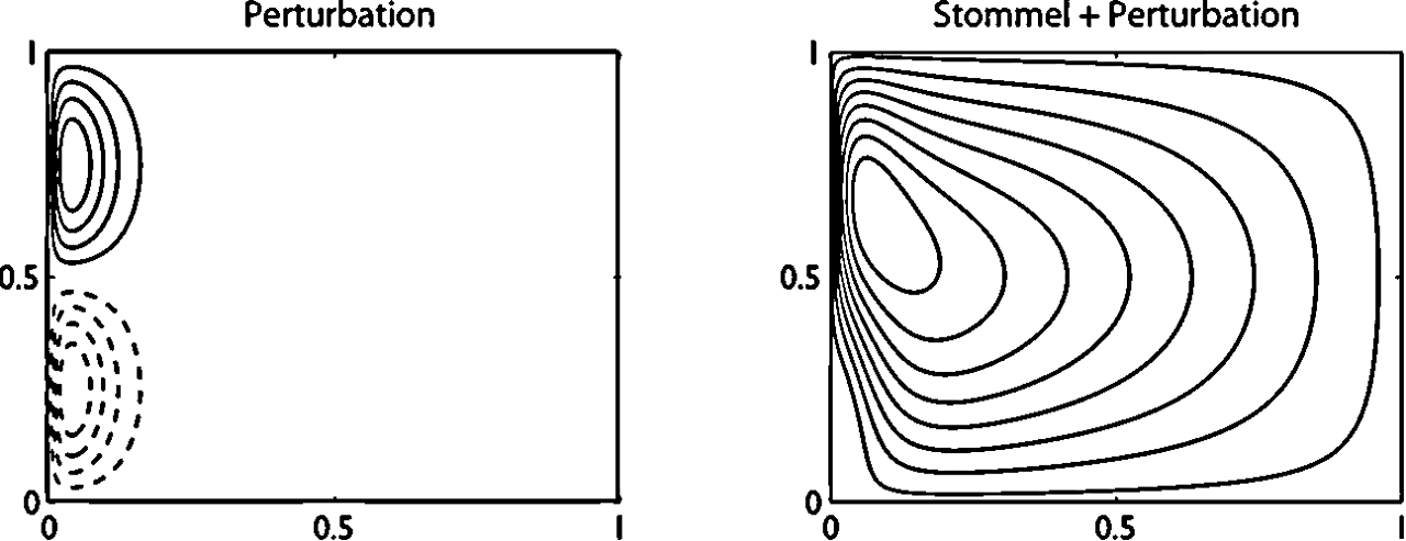
The nonlinear perturbation solution of the Stommel problem. On the left is the perturbation
$
-\frac{R_\beta \pi^3}{2 \epsilon_S^3} \sin(2\pi y) x e^{-x/\epsilon_S}
$,
and on the right is the reconstituted solution.
Dashed contours are negative
1Vallis, G.K. (2017) Atmospheric and Oceanic Fluid Dynamics: Fundamentals and Large-Scale Circulation. 2nd edn. Cambridge: Cambridge University Press.