The basic algorithm employed for stepping forward the momentum equations is based on retaining non-divergence of the flow at all times. This is most naturally done if the components of flow are staggered in space in the form of an Arakawa C grid.

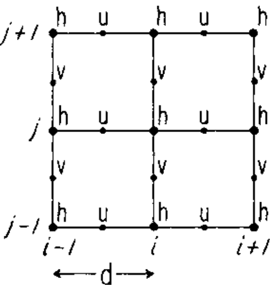
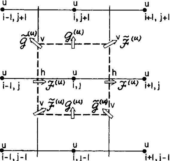
(1) Simulate the 2D linearised rotating shallow-water equations on a square domain using an Arakawa C-grid: initialize a cell-centered geopotential field with a localized positive perturbation at the domain center (zero elsewhere), define staggered zonal and meridional velocities on the C-grid, and advance the coupled system forward in time with an explicit scheme using second-order centered finite differences (including Coriolis coupling and appropriate velocity averaging for interpolation). Report the gravity-wave Courant number for the chosen grid spacing and time step, and visualize the evolving geopotential field together with the velocity field (e.g., using contourf/imshow for height and arrows/streamlines for velocity) over several time steps to illustrate wave propagation and the flow response to the initial perturbation.

(2) Implement the linearised rotating shallow-water equations on an Arakawa A-grid or Arakawa B-grid using the same numerical parameters as in the C-grid case. Compare the solutions obtained with different grid staggers and discuss any differences.