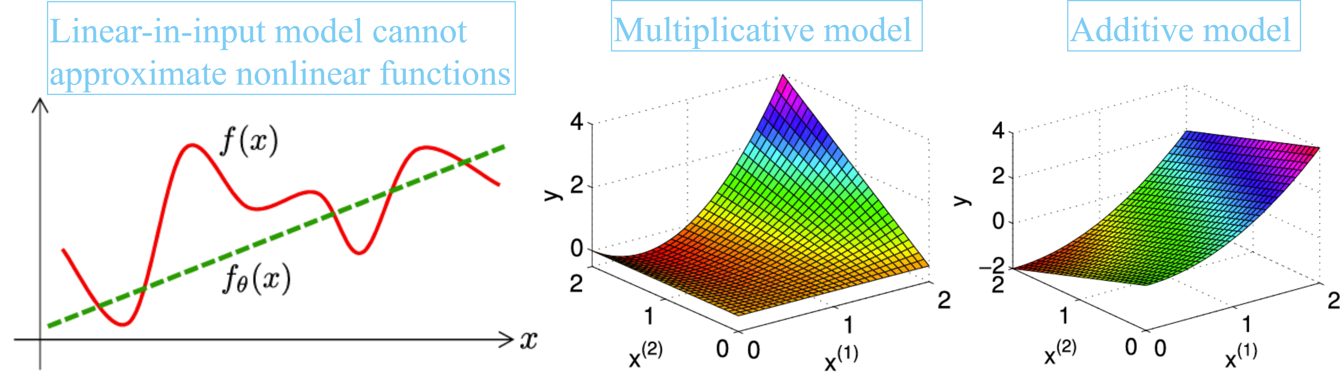
For simplicity, let us begin with a one-dimensional learning target function $f$. The simplest model for approximating $f$ would be the linear-in-input model $\theta \times x$. Here, $\theta$ denotes a scalar parameter and the target function is approximated by learning the parameter $\theta$. Although the linear-in-input model is mathematically easy to handle, it can only approximate a linear function (i.e., a straight line) and thus its expression power is limited

The linear-in-parameter model is an extension of the linear-in-input model that allows approximation of nonlinear functions: \[ f_\theta(x) = \sum_{j=1}^{b} \theta_j \phi_j(x) \] where $\phi_j(x)$ and $\theta_j$ are a basis function and its parameter, respectively, and $b$ denotes the number of basis functions. The linear-in-parameter model may be compactly expressed as \[ f_\theta(x) = \theta^\top \phi(x) \] where \[ \phi(x) = (\phi_1(x), \ldots, \phi_b(x))^\top \]