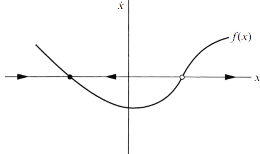
To any one-dimensional system \(\dot{x} = f(x)\), just need to draw the graph of \(f(x)\) and then use it to sketch the vector field on the real line
Imagine that a fluid is flowing along the real line with a local velocity \(f(x)\). This imaginary fluid is called the phase fluid, and the real line is the phase space. The flow is to the right where \(f(x) > 0\) and to the left where \(f(x) < 0\). To find the solution to \(\dot{x} = f(x)\) starting from an arbitrary initial condition \(x_0\), place an imaginary particle (a phase point) at \(x_0\) and watch how it is carried along by the flow. As time goes on, the phase point moves along the \(x\)-axis according to some function \(x(t)\).
This function is called the trajectory based at \(x_0\), and it represents the solution of the differential equation starting from the initial condition \(x_0\). A figure shows all the qualitatively different trajectories of the system is called a phase portrait
The appearance of the phase portrait is controlled by the fixed points \(x^*\), defined by \(f(x^*) = 0\); they correspond to stagnation points of the flow. \(\boxed{\text{ fixed points} = \begin{cases} \text{stable (attractor, sink)} \\ \text{unstable (repeller, source)} \end{cases}} \)
- The solid black dot is a stable fixed point (the local flow is toward it)
- The open dot is an unstable fixed point (the flow is away from it)
1Strogatz, S.H. (2015). Nonlinear Dynamics and Chaos: With Applications to Physics, Biology, Chemistry, and Engineering (2nd ed.). CRC Press.