One of the most basic techniques of dynamics: interpreting a differential equation as a vector field
Consider \(\dot{x} = \sin x\)
Separate the variables and then integrate: \(dt = \frac{dx}{\sin x}\)
\(\Rightarrow dt = \frac{dx}{\sin x}, dt = \csc x \, dx \Rightarrow \int dt = \int \csc x \, dx \Rightarrow t = \int \csc x \, dx \)
which implies \(t = \int \csc x \, dx = -\ln|\csc x + \cot x| + C\)
To evaluate the constant \( C \), suppose \( x = x_0 \) at \( t = 0 \)
Then \( C = \ln |\csc x_0 + \cot x_0| \)
Hence the solution is \(t = \ln \left| \frac{\csc x_0 + \cot x_0}{\csc x + \cot x} \right|\)
This result is exact, but a headache to interpret
\[ \dot{x} = \sin x \]
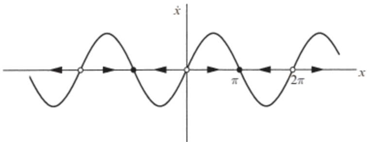
Think of \( t \) as time, \( x \) as the position of an imaginary particle moving along the real line, and \( \dot{x} \) as the velocity of that particle. Then the differential equation \( \dot{x} = \sin x \) represents a vector field on the line: it dictates the velocity vector \( \dot{x} \) at each \( x \). To sketch the vector field, it is convenient to plot \( \dot{x} \) versus \( x \), and then draw arrows on the \( x \)-axis to indicate the corresponding velocity vector at each \( x \)
The arrows point to the right when \( \dot{x} > 0 \) and to the left when \( \dot{x} < 0 \)
1Some food for thought: Strogatz, S.H. (2015). Nonlinear Dynamics and Chaos: With Applications to Physics, Biology, Chemistry, and Engineering (2nd ed.). CRC Press.