From 1D to 2D systems, fixed points can still be created or destroyed or destabilized as parameters are varied — but now the same is true of closed orbits as well. We can begin to describe the ways in which oscillations can be turned on or off
Examples
- \(\dot{x} = \mu x - x^2,\quad \dot{y} = -y \qquad\qquad\quad (\text{transcritical})\)
- \(\dot{x} = \mu x - x^3,\quad \dot{y} = -y \qquad\qquad\quad (\text{supercritical pitchfork})\)
- \(\dot{x} = \mu x + x^3,\quad \dot{y} = -y \qquad\qquad\quad (\text{subcritical pitchfork})\)
The bifurcation points so far have one common feature. All the branches have represented equilibria — both branches intersecting in a bifurcation point have consisted of (stationary) solutions of the equation \(\boxed{\dot{\mathbf{y}} = 0 = \mathbf{f}(\mathbf{y},\lambda)}\). A bifurcation that is characterized by intersecting branches of equilibrium points stationary bifurcation (also called steady-state bifurcation)
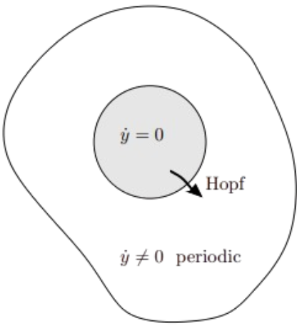
The corresponding function spaces of \(\mathbf{y}(t)\) include equilibria as the special-case constant solutions. The type of bifurcation that connects equilibria with periodic motion is Hopf bifurcation. Hopf bifurcation is the door that opens from the small room of equilibria to the large hall of periodic solutions, which in turn is just a small part of the realm of functions
1Strogatz, S.H. (2015). Nonlinear Dynamics and Chaos: With Applications to Physics, Biology, Chemistry, and Engineering (2nd ed.). CRC Press.
2Seydel, R. (2010). Practical Bifurcation and Stability Analysis. Interdisciplinary Applied Mathematics, vol 5. Springer, New York, NY.