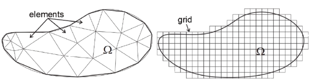
The Finite Element method is similar to the Finite Volume method in many ways. The domain is broken into a set of discrete volumes or finite elements that are generally unstructured

• In 2D, they are usually triangles or quadrilaterals
• In 3D tetrahedra or hexahedra are most often used

The distinguishing feature of Finite Element methoda is that the equations are multiplied by a weight function before they are integrated over the entire domain. In the simplest Finite Element method, the solution is approximated by a linear shape function within each element in a way that guarantees continuity of the solution across element boundaries. Such a function can be constructed from its values at the corners of the elements. The weight function is usually of the same form

This approximation is then substituted into the weighted integral of the conservation law and the equations to be solved are derived by requiring the derivative of the integral with respect to each nodal value to be zero; this corresponds to selecting the best solution within the set of allowed functions (the one with minimum residual). The result is a set of non-linear algebraic equations

An important advantage of finite element methods is the ability to deal with arbitrary geometries

• There is an extensive literature devoted to the construction of grids for finite element methods
• The grids are easily refined; each element is simply subdivided
• Finite element methods are relatively easy to analyze mathematically and can be shown to have optimality properties for certain types of equations

A hybrid method called control-volume-based finite element method (CVFEM) should also be mentioned. In it, shape functions are used to describe the variation of the variables over an element. Control volumes are formed around each node by joining the centroids of the elements. The conservation equations in integral form are applied to these CVs in the same way as in the finite volume method. The fluxes through CV boundaries and the source terms are calculated element-wise