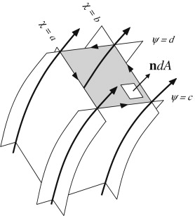
The mass flux \( \dot{m} \) through the surface \( A \) bounded by the four stream surfaces (shown in gray) is calculated with area element \( dA \), normal \( \mathbf{n} \) (as shown), and Stokes’ theorem
Defining the mass flux \( \dot{m} \) through \( A \), and using Stokes’ theorem produces \[ \dot{m} = \int_A \rho \mathbf{u} \cdot \mathbf{n} \, dA = \int_A (\nabla \times \mathbf{\Psi}) \cdot \mathbf{n} \, dA = \int_C \mathbf{\Psi} \cdot d\mathbf{s} = \int_C \chi \nabla \psi \cdot d\mathbf{s} = \int_C \chi \, d\psi \] \[ = b(d - c) + a(c - d) = (b - a)(d - c) \]

Here we have used the vector identity \( \boxed{\nabla \psi \cdot d\mathbf{s} = d\psi} \) The mass flow rate of the stream tube defined by adjacent members of the two families of stream functions is just the product of the differences of the numerical values of the respective stream functions

As a special case, consider two-dimensional flow in \((x, y)\)-Cartesian coordinates where all the streamlines lie in \( z = \text{constant} \) planes. In this situation \( z \) is one of the three-dimensional stream functions, so we can set \( \chi = -z \), where the sign is chosen to obey the usual convention. This produces \( \nabla \chi = -\mathbf{e}_z \), so \( \rho \mathbf{u} = -\mathbf{e}_z \times \nabla \psi \), or \[ \rho u = \frac{\partial \psi}{\partial y}, \quad \rho v = -\frac{\partial \psi}{\partial x} \]

[Q] Write out all the components of the stress tensor \(\mathbf{T}\) in \((x, y, z)\)-coordinates in terms of \( \mathbf{u} = (u, v, w) \) and its derivatives

[Sol] Evaluate each component of the stress tensor \(T_{ij} = -p \delta_{ij} + \tau_{ij} = -p \delta_{ij} + 2\mu \left( S_{ij} - \frac{1}{3} S_{mm} \delta_{ij} \right) + \mu_v S_{mm} \delta_{ij}\) and abbreviate \( S_{mm} = \frac{\partial u}{\partial x} + \frac{\partial v}{\partial y} + \frac{\partial w}{\partial z} = \nabla \cdot \mathbf{u} \) to find \[ \mathbf{T} = \begin{bmatrix} -p + 2\mu \frac{\partial u}{\partial x} + \left( \mu_v - \frac{2}{3} \mu \right) \nabla \cdot \mathbf{u} & \mu \left( \frac{\partial u}{\partial y} + \frac{\partial v}{\partial x} \right) & \mu \left( \frac{\partial u}{\partial z} + \frac{\partial w}{\partial x} \right) \\ \mu \left( \frac{\partial v}{\partial x} + \frac{\partial u}{\partial y} \right) & -p + 2\mu \frac{\partial v}{\partial y} + \left( \mu_v - \frac{2}{3} \mu \right) \nabla \cdot \mathbf{u} & \mu \left( \frac{\partial v}{\partial z} + \frac{\partial w}{\partial y} \right) \\ \mu \left( \frac{\partial w}{\partial x} + \frac{\partial u}{\partial z} \right) & \mu \left( \frac{\partial w}{\partial y} + \frac{\partial v}{\partial z} \right) & -p + 2\mu \frac{\partial w}{\partial z} + \left( \mu_v - \frac{2}{3} \mu \right) \nabla \cdot \mathbf{u} \end{bmatrix} \] \(\rho u = \frac{\partial \psi}{\partial y}, \rho v = -\frac{\partial \psi}{\partial x}\) in conformity with \(\boxed{ \mathbf{T} = \begin{bmatrix} -p + \frac{2\mu}{\rho} \frac{\partial^2 \psi}{\partial x \partial y} & \frac{\mu}{\rho} \left( \frac{\partial^2 \psi}{\partial y^2} - \frac{\partial^2 \psi}{\partial x^2} \right) \\ \frac{\mu}{\rho} \left( \frac{\partial^2 \psi}{\partial y^2} - \frac{\partial^2 \psi}{\partial x^2} \right) & -p - \frac{2\mu}{\rho} \frac{\partial^2 \psi}{\partial x \partial y} \end{bmatrix}} \)

◀ ▶