Stable and Unstable Mechanical Systems: Example
For the given initial conditions, the solution for \( x(t) \) is: \[ x(t) = A e^{\beta_- t} + B e^{\beta_+ t}, \quad \text{where } \beta_{\pm} = -\frac{\gamma}{2m} \pm \sqrt{ \frac{\gamma^2}{4m^2} - \frac{k_s}{m} } \]
There are three distinct cases:
- If \( \gamma > 0 \) and \( k_s > 0 \), then \( x(t) \) is stable because both \( \beta_+ \) and \( \beta_- \) will have negative real parts and the initial displacement decays exponentially with increasing time
- If \( k_s = 0 \), then \( \beta_+ \) will be zero for any value of \( \gamma \), and the solution for \( x(t) \) reduces to \( x = \varepsilon \). This represents neutral stability since a new steady solution emerges after the initial displacement
- If \( \gamma < 0 \) and \( k_s > 0 \), then \( x(t) \) is unstable since both \( \beta_+ \) and \( \beta_- \) have a positive real part and the initial displacement grows exponentially with increasing time
Interestingly, real fluid flows can mimic this negative-damping destabilizing effect
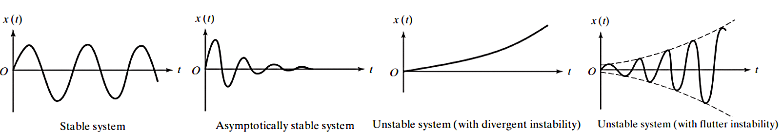
Different types of stability
1Rao, S.S. (2006) Mechanical Vibration. 5th Edition, Pearson Education, Inc., Upper Saddle River, 603-606.