Computers work with discrete numbers so we must approximate the continuous flow field by discrete values and the partial differential equations must be replaced by discrete equations that relate the discrete values to each other. There are several ways to do so but here we will focus on two approaches:
- Finite differences: start with the governing equations in differential form and approximate the continuum equations for the values at each point by approximate formula for the various derivatives, usually using a Taylor series expansion
- Finite volumes: divide the flow domain into small control volumes and use the governing equations in integral form to derive discrete approximate equations for the average values in each control volume
In both cases the grid must be sufficiently fine so that the velocity, pressure, and other variables in each control volume, or in between the points, are well described by simple functions determined by one or few parameters. The discrete equations are then used to determine these parameters
The Figure shows the general idea. The domain where we need to find the flow is divided by a grid that defines small control volumes or connected grid points. The grid must be sufficiently fine so that the velocity does not change much from one grid point or control volume to the next. principles of conservation of mass, momentum, and energy are then applied to each control volume or a grid point to find the point wise or the average velocity.
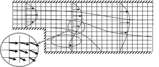
The approximation of a flow field on a discrete grid, where the grid points are either where we approximate the equations using finite differences or the centers of small control volumes. The horizontal component of the fluid velocity at three cross-sections and a few streamlines are shown.