When computing unsteady flows, we have a fourth coordinate direction to consider: time. Just as with the space coordinates, time must be discretized. We can consider the time “grid” in either the finite difference spirit, as discrete points in time, or in a finite volume view as “time volumes”

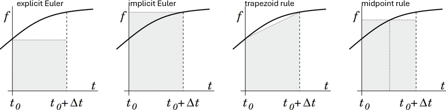
The simplest method is explicit Euler in which all fluxes and sources are evaluated using known values at $t_n$. In the equation for a control volume or grid point, the only unknown at the new time level is the value at that node; the neighbor values are all evaluated at earlier time levels. Thus one can explicitly calculate the new value of the unknown at each node.

These methods are very similar to ones applied to initial value problems for ordinary differential equations (ODEs)

◀ ▶