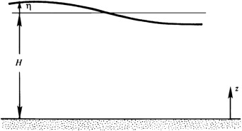
Consider a homogeneous layer of fluid of average depth \(H\) lying over a flat horizontal bottom. Set \(z = 0\) on the bottom surface, and let \(\eta(x, y, t)\) be the displacement of the free surface. When the pressure on the fluid's surface is set to zero, the pressure at height \(z\) from the bottom, which is hydrostatic, is given by \[p = \rho g \left( H + \eta(x, y, t) - z \right)\] so the pressure gradient is: \[\nabla p = \mathbf{e}_x \, \rho g \left( \frac{\partial \eta}{\partial x} \right) + \mathbf{e}_y \, \rho g \left( \frac{\partial \eta}{\partial y} \right) - \mathbf{e}_z \, \rho g\]

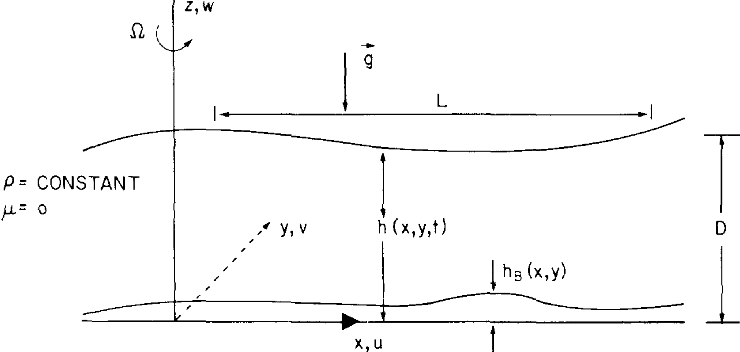
With application to the earth’s atmosphere or ocean in mind, model the body force arising from the potential \(\Phi\) as a vector, \(\mathbf{g}\), directed perpendicular to the \(z = 0\) surface.

The rotation axis of the fluid coincides with the \(z\)-axis in the model \(\boldsymbol{\Omega} = \mathbf{k} \Omega\), so that in this case the Coriolis parameter \(f\) is simply \(2\Omega\).

The rigid bottom is defined by the surface \(z = h_B(x, y)\). The velocity has components \(u, v,\) and \(w\) parallel to the \(x\)-, \(y\)-, and \(z\)-axes respectively. The pressure of the fluid surface can be arbitrarily imposed, but for our purposes we may take it to be constant.