Given the ease with which it can be measured, the pressure below the liquid surface is considered first. In particular, the time-dependent perturbation pressure
\[
p' \equiv p + \rho g z
\]
produced by surface waves is of interest
\(\because\) \(p' \equiv p + \rho g z\) and \(\phi = \frac{a \omega}{k} \frac{\cosh(k(z + H))}{\sinh(kH)} \sin(kx - \omega t)\) in the linearized Bernoulli equation \(\frac{\partial \phi}{\partial t} + \frac{p}{\rho} + gz \cong 0\)
\(\therefore\) \(p' = -\rho \frac{\partial \phi}{\partial t}
= \rho \frac{\omega^2 a}{k} \frac{\cosh(k(z+H))}{\sinh(kH)} \cos(kx - \omega t)
= \rho g a \frac{\cosh(k(z+H))}{\cosh(kH)} \cos(kx - \omega t)\)
The \(\boxed{\rho \frac{\omega^2 a}{k} \frac{\cosh(k(z+H))}{\sinh(kH)} \cos(kx - \omega t)
= \rho g a \frac{\cosh(k(z+H))}{\cosh(kH)} \cos(kx - \omega t)}\) in it follows when \(\omega = \sqrt{gk \tanh(kH)} \quad \text{or} \quad T = \sqrt{\frac{2\pi \lambda}{g} \coth\left(\frac{2\pi H}{\lambda}\right)}\) is used to eliminate \(\omega^2\)
The perturbation pressure decreases with increasing depth, and the extent of this decrease depends on the wavelength through \(k\)
Another interesting feature of linear surface waves is the fact that they travel and cause fluid elements to move, but they do not cause fluid elements to travel, when a linear surface wave passes, consider the fluid element that follows a path
\(
\mathbf{x}_p(t) = x_p(t)\mathbf{e}_x + z_p(t)\mathbf{e}_z
\)
The path-line equations for this fluid element are
\[
\frac{dx_p(t)}{dt} = u(x_p, z_p, t) \quad \text{and} \quad \frac{dz_p(t)}{dt} = w(x_p, z_p, t)
\]
With the fluid velocity components \(u = \omega a \frac{\cosh(k(z + H))}{\sinh(kH)} \cos(kx - \omega t) \text{ and } w = \omega a \frac{\sinh(k(z + H))}{\sinh(kH)} \sin(kx - \omega t)\)
\(\Rightarrow
\frac{dx_p}{dt} = \omega a \frac{\cosh(k(z_p+H))}{\sinh(kH)} \cos(kx_p - \omega t),
\frac{dz_p}{dt} = \omega a \frac{\sinh(k(z_p+H))}{\sinh(kH)} \sin(kx_p - \omega t)
\)
To be consistent with the small amplitude approximation, these equations can be linearized by setting
\[
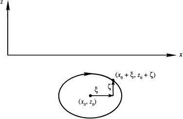
x_p(t) = x_0 + \xi(t) \quad \text{and} \quad z_p(t) = z_0 + \zeta(t)
\]
where \((x_0, z_0)\) is the average fluid element location and the element excursion vector \((\xi, \zeta)\) is assumed to be small compared to the wavelength
\(\therefore\) The linearized versions are obtained by evaluating the right side of each equation at \((x_0, z_0)\) assumed independent of time:
\[ \frac{d\xi}{dt} \cong \omega a \frac{\cosh(k(z_0+H))}{\sinh(kH)} \cos(kx_0 - \omega t) \quad \text{and} \quad \frac{d\zeta}{dt} \cong \omega a \frac{\sinh(k(z_0+H))}{\sinh(kH)} \sin(kx_0 - \omega t)\] ◀ ▶